Source: Parker et al. (1997). Copyright 1997 by Fairmont Press, Inc., 700 Indian Trail, Lilburn, GA 30047, www.fairmontpress.com. Reprinted by permission from Energy Management Handbook.
Carbon monoxide upper control limits vary with the boiler fuel used. The CO limit for gas-fired boilers may be set typically at 400, 200, or 100 ppm. For No. 2 fuel oil, the maximum SSN is typically 1; for No. 6 fuel oil, SSN = 4. However, for any fuel used, local environmental regulations may require lower limits.
To maintain safe unit output conditions, excess air requirements may be greater than the levels indicated in this table. This condition may arise when operating loads are substantially less than the design rating. Where possible, the vendor’s predicted performance curves should be checked. If they are unavailable, excess air should be reduced to minimum levels consistent with satisfactory output.
Oxygen Trim Control
An oxygen trim control system adjusts the airflow rate using an electromechanical actuator mounted on the boiler’s forced-draft fan damper linkage, and measures excess oxygen using a zirconium oxide mounted in the boiler stack. The oxygen sensor signal is compared with a set point value obtained from the boiler’s excess air set point curve for the given firing rate. The oxygen trim controller adjusts (“trims”) the damper setting to regulate the oxygen level in the boiler stack at this set point. In the event of an electronic failure, the boiler defaults to the air setting determined by the mechanical linkages.
Carbon Monoxide Trim Control
Carbon monoxide trim control systems are also used to control excess air, and offer several advantages over oxygen trim systems. In carbon monoxide trim systems, the amount of unburned fuel (in the form of carbon monoxide) in the flue gas is measured directly by a carbon monoxide sensor and the air/fuel ratio control is set to actual combustion conditions rather than preset oxygen levels. Thus, the system continuously controls for minimum excess air. Carbon monoxide trim systems are also independent of fuel type and are virtually unaffected by combustion air temperature, humidity, and barometric pressure conditions. However, they cost more than oxygen trim systems because of the expense of the carbon monoxide sensor. Also, the carbon monoxide level in the boiler stack is not always a measure of excess air. A dirty burner, poor atomization, flame chilling, flame impingement on the boiler tubes, or poor fuel mixing can also raise the carbon monoxide level in the boiler stack (Taplin 1998).
Sequencing and Loading of Multiple Boilers
Generally, boilers operate most efficiently at a 65 to 85% full-load rating. Boiler efficiencies fall off at higher and lower load points, with the decrease most pronounced at low load conditions. Boiler efficiency can be calculated by means of stack temperature and percent O2 (or percent excess air) in the boiler stack for a given fuel type. Part-load curves of boiler efficiency versus hot-water or steam load should be developed for each boiler. These curves should be dynamically updated at discrete load levels based on the hot-water or steam plant characteristics to allow the control strategy to continuously predict the input fuel requirement for any given heat load. When the hot-water temperature or steam pressure drops below set point for the predetermined time interval (e.g., 5 min), the most efficient combination of boilers must be selected and turned on to meet the load. The least efficient boiler should be shut down and banked in hot standby if its capacity drops below the spare capacity of the current number of boilers operating (or for primary/secondary hot-water systems, if the flow rate of the associated primary hot-water pump is less than the difference between primary and secondary hot-water flow rates) for a predetermined time interval (e.g., 5 min). The spare capacity of the current online boilers is equal to their full-load capacity minus the current hot water load.
Resetting Supply Water Temperature and Pressure
Standby losses are reduced and overall efficiencies enhanced by operating hot-water boilers at the lowest acceptable temperature. Condensing boilers achieve significantly higher combustion efficiencies at water temperatures below the dew point when they are operating in condensing mode (Chapter 27, Boilers, in the 2004 ASHRAE Handbook—HVAC Systems and Equipment). Hot-water boilers of this type are very efficient at part-load operation when a high water temperature is not required. Energy savings are therefore possible if the supply water temperature is maintained at the minimum level required to satisfy the largest heating load. However, to minimize condensation of flue gases and consequent boiler damage from acid, water temperature should not be reset below that recommended by the boiler manufacturer (typically 140°F).
Similarly, energy can be saved in steam heating systems by maintaining supply pressure at the minimum level required to satisfy the largest heating load.
In practice, reset control is only possible if boiler controls interface with the energy management and control system.
Operating Constraints
Note that there are practical limitations on the extent of automatic operation if damage to the boiler is to be prevented. Control strategies to reduce boiler energy consumption can also conflict with recommended boiler operating practice. For example, in addition to flue gas condensation concerns mentioned previously, rapid changes in boiler metal temperature (thermal shock) brought about by abrupt changes in boiler water temperature or flow, firing rate, or air temperature entering the boiler should be avoided. The repeated occurrence of these conditions weakens the metal and leads to cracking and/or loose tubes. It is therefore important to follow all of the recommendations of the American Boiler Manufacturers Association (ABMA 1998).
Controls for Cooling Without Storage
Figure 1 depicts multiple chillers, cooling towers, and pumps providing chilled water to air-handling units to cool air that is supplied to building zones. At any given time, cooling needs may be met with different modes of operation and set points. However, one set of control set points and modes results in minimum power consumption. This optimal control point results from tradeoffs between the energy consumption of different components. For instance, increasing the number of cooling tower cells (or fan speeds) increases fan power but reduces chiller power because the temperature of the water supplied to the chiller’s condenser is decreased. Similarly, increasing condenser water flow by adding pumps (or increasing pump speed) decreases chiller power but increases pump power.
Similar tradeoffs exist for the chilled-water loop variables of systems with variable-speed chilled-water pumps and air handler fans. For instance, increasing the chilled-water set point reduces chiller power but increases pump power because greater flow is needed to meet the load. Increasing the supply air set point increases fan power, but decreases pump power.
Figure 8 illustrates the sensitivity of the total power consumption to condenser water-loop controls (from Braun et al. 1989a) for a single chiller load, ambient wet-bulb temperature, and chilled-water supply temperature. Contours of constant power consumption are plotted versus cooling tower fan and condenser water pump speed for a system with variable-speed fans and pumps. Near the optimum, power consumption is not sensitive to either of these control variables, but increases significantly away from the optimum. The rate of increase in power consumption is particularly large at low condenser pump speeds. A minimum pump speed is necessary to overcome the static pressure associated with the height of the water discharge in the cooling tower above the sump. As the pump speed approaches this value, condenser flow approaches zero and chiller power increases dramatically. A pump speed that is too high is generally better than one that is too low. The broad area near the optimum indicates that, for a given load, the optimal setting does not need to be accurately determined. However, optimal settings change significantly when there are widely varying chiller loads and ambient wet-bulb temperature.
Figure 9 illustrates the sensitivity of power consumption to chilled-water and supply air set-point temperatures for a system with variable-speed chilled-water pumps and air handler fans (from Braun et al. 1989a). Within about 3°F of the optimum values, the power consumption is within 1% of the minimum. Outside this range, sensitivity to the set points increases significantly. The penalty associated with operation away from the optimum is greater in the direction of smaller differences between the supply air and chilled-water set points. As this temperature difference is reduced, the required flow of chilled water to this coil increases and the chilled-water pumping power is greater. For a given chilled-water or supply air temperature, the temperature difference is limited by the heat transfer characteristics of the coil. As this limit is approached, the required water flow and pumping power would become infinite if the pump speed were not constrained. It is generally better to have too large rather than too small a temperature difference between the supply air and chilled-water set points.
For constant chilled-water flow, the tradeoffs in energy use with chilled-water set point are very different than for variable-flow systems. Increasing the chilled-water set point reduces chiller power consumption, but has little effect on chilled-water pumping energy. Therefore, the benefits of chilled-water temperature reset are more significant than for variable-flow systems (although variable-flow systems use less energy). For constant chilled-water flow, the minimum-cost strategy is to raise the chilled-water set point to the highest value that will keep all discharge air temperatures at their set points and keep zone humidities within acceptable bounds.
For constant-volume (CAV) air-handling systems, the tradeoffs in energy use with supply air set point are also very different than for variable air volume systems. Increasing the supply air set point for cooling reduces both the cooling load and reheat required, but does not change fan energy. Again, the benefits of supply air temperature reset for CAV systems are more significant than for VAV systems (although VAV systems use less energy). In general, the set point for a CAV system should be set at the highest value that will keep all zone temperatures at their set points and all humidities within acceptable limits.
In addition to the set points used by local-loop controllers, a number of operational modes can affect performance. For instance, significant energy savings are possible when a system is properly switched over to an economizer cycle. At the onset of economizer operation, return dampers are closed, outside dampers are opened, and the maximum possible outside air is supplied to cooling coils. Two different types of switchover are typically used: (1) dry-bulb and (2) enthalpy. With a dry-bulb economizer, the switchover occurs when the ambient dry-bulb temperature is less than a specified value, typically between 55 and 65°F. With an enthalpy economizer, the switchover typically happens when the outdoor enthalpy (or wet-bulb temperature) is less than the enthalpy (or wet-bulb temperature) of the return air. Although the enthalpy economizer yields lower overall energy consumption, it requires wet-bulb temperature or dry-bulb and relative humidity measurements.
Another important operation mode is the sequencing of chillers and pumps. Sequencing defines the order and conditions associated with bringing equipment online or offline. Optimal sequencing depends on the individual design and part-load performance characteristics of the equipment. For instance, more-efficient chillers should generally be brought online before less-efficient ones. Furthermore, the conditions where chillers and pumps should be brought online depend on their performance characteristics at part-load conditions.
Figure 10 shows an example of optimal system performance (i.e., optimal set-point choices) for different combinations of chillers and fixed-speed pumps in parallel as a function of load relative to the design load for a given ambient wet-bulb temperature. For this system (from Braun et al. 1989a), each component (chillers, chilled-water pumps, and condenser water pumps) in each parallel set is identical and sized to meet half of the design requirements. The best performance occurs at about 25% of the design load with one chiller and pump operating. As the load increases, the system COP decreases because of decreasing chiller COP and a nonlinear increase in the power consumption of cooling tower and air handler fans. A second chiller should be brought online at the point where the overall COP of the system is the same with or without the chiller. For this system, this optimal switch point occurs at about 38% of the total design load or about 75% of the individual chiller’s capacity. The optimal switch point for bringing a second condenser and chilled-water pump online occurs at a much higher relative chilled load (0.62) than the switch point for adding or removing a chiller (0.38). However, pumps are typically sequenced with chillers (i.e., they are brought online together). In this case, Figure 7 shows that the optimal switch point for bringing a second chiller online (with pumps) is about 50% of the overall design load or at the design capacity of the individual chiller. This is generally the case for sequencing chillers with dedicated pumps.
In most cases, zone humidities are allowed to float between upper and lower limits dictated by comfort (see Chapter 8, Thermal Comfort, of the 2009 ASHRAE Handbook—Fundamentals). However, VAV systems can control the zone humidity and temperature simultaneously. For a zone being cooled, the equipment operating costs are minimized when the zone temperature is at the upper bound of the comfort region. However, operating simultaneously at the upper limit of humidity does not minimize operating costs. Figure 11 shows an example comparison of system COP and zone humidity associated with fixed and free-floating zone humidity as a function of the relative load (from Braun et al. 1989a). Over the range of loads, allowing the humidity to float within the comfort zone produces a lower cost and zone humidity than setting the humidity at the highest acceptable value. The largest differences occur at the highest loads. Operation with the zone at the upper humidity bound results in lower latent loads than with a free-floating humidity, but this humidity control constraint requires a higher supply air temperature, which in turn results in greater air handler power consumption. For minimum energy costs, the humidity should be allowed to float freely within the bounds of human comfort.
Effects of Load and Ambient Conditions on Optimal Supervisory Control
When the ratio of individual zone loads to total load does not change significantly with time, the optimal control variables are functions of the total sensible and latent gains to the zones and of the ambient dry- and wet-bulb temperatures. For systems with wet cooling towers and climates where moisture is removed from conditioned air, the effect of the ambient dry-bulb temperature alone is small because air enthalpy depends primarily on wet-bulb temperature, and the performance of wet-surface heat exchangers is driven primarily by the enthalpy difference. Typically, zone latent gains are on the order of 15 to 25% of the total zone gains, and changes in latent gains have a relatively small effect on performance for a given total load. Consequently, in many cases optimal supervisory control variables depend primarily on ambient wet-bulb temperature and total chilled-water load. However, load distributions between zones may also be important if they change significantly over time.
Generally, optimal chilled-water and supply air temperatures decrease with increasing load for a fixed ambient wet-bulb temperature and increase with increasing ambient wet-bulb temperature for a fixed load. Furthermore, optimal cooling tower airflow and condenser water flow rates increase with increasing load and ambient wet-bulb temperature.
Performance Comparisons for Supervisory Control Strategies
Optimization of plant operation is most important when loads vary and when operation is far from design conditions for a significant period. Various strategies are used for chilled-water systems at off-design conditions. Commonly, the chilled-water and supply air set-point temperatures are changed only according to the ambient dry-bulb temperature. In some systems, cooling tower airflow and condenser water flow are not varied in response to changes in the load and ambient wet-bulb temperature. In other systems these flow rates are controlled to maintain constant temperature differences between the cooling tower outlet and the ambient wet-bulb temperature (approach) and between the cooling tower inlet and outlet (range), regardless of the load and wet-bulb temperature. Although these strategies seem reasonable, they do not generally minimize operating costs.
Figure 12 shows a comparison of the COPs for optimal control and three alternative strategies as a function of load for a fixed ambient wet-bulb temperature. This system (from Braun et al. 1989a) incorporated the use of variable-speed pumps and fans. The three strategies are
- Fixed chilled-water and supply air temperature set points (40 and 52°F, respectively), with optimal condenser-loop control
- Fixed tower approach and range (5 and 12°F, respectively), with optimal chilled-water loop control
- Fixed set points, approach, and range
Because the fixed values were chosen to be optimal at design conditions, the differences in performance for all strategies are minimal at high loads. However, at part-load conditions, Figure 12 shows that the savings associated with the use of optimal control can become significant. Optimal control of the chilled-water loop results in greater savings than that for the condenser loop for part-load ratios less than about 50%. The overall savings over a cooling season depend on the time variation of the load. If the cooling load is relatively constant and near the design load, fixed values of temperature set points, approach, and range could be chosen to give near-optimal performance. However, for typical building loads with significant daily and seasonal variations, the penalty for using a fixed set-point control strategy is typically in the range of 5 to 20% of the cooling system energy.
Even greater energy savings are possible with economizer control and discharge air temperature reset with constant-volume systems. Kao (1985) investigated the effect of different economizer and supply air reset strategies on both heating and cooling energy use for CAV, VAV, and dual-duct air handling systems for four different buildings. The results indicated that substantial improvements in a building’s energy use may be obtained.
Variable- Versus Fixed-Speed Equipment
Using variable-speed motors for chillers, fans, and pumps can significantly reduce energy costs but can also complicate the problem of determining optimal control. The overall savings from using variable-speed equipment over a cooling season depend on the time variation of the load. Typically, using variable-speed drives reduces equipment operating costs 20 to 50% compared to equipment with fixed-speed drives.
Figure 13 gives the overall optimal system performance for a cooling plant with either variable-speed or fixed-speed, variable-vane control of a centrifugal chiller. At part-load conditions, the system COP associated with using a variable-speed chiller is improved as much as 25%. However, the power requirements are similar at conditions associated with peak loads, because at full load the vanes are wide open and the speed under variable-speed control and fixed-speed operation is the same. The results of Figure 10 are from a single case study of a large chilled-water facility at the Dallas/Ft. Worth Airport (Braun et al. 1989a), constructed in the mid-1970s, where the existing chiller was retrofitted with a variable-speed drive. Differences in performance between variable- and fixed-speed chillers may be smaller for current equipment.
The most common design for cooling towers places multiple tower cells in parallel with a common sump. Each tower cell has a fan with one, two, or possibly three operating speeds. Although multiple cells with multiple fan settings offer wide flexibility in control, the use of variable-speed tower fans can provide additional improvements in overall system performance. Figure 14 shows an example comparison of optimal performance for single-speed, two-speed, and variable-speed tower fans as a function of load for a given wet-bulb temperature for a system with four cells (Braun et al. 1989a). The variable-speed option results in higher COP under all conditions. In contrast, for discrete fan control, the tower cells are isolated when their fans are off and the performance is poorer. Below about 70% of full-load conditions, there is a 15% difference in total energy consumption between single-speed and variable-speed fans. Between two-speed and variable-speed fans, the differences are much smaller, about 3 to 5% over the entire range.
Fixed-speed pumps that are sized to give proper flow to a chiller at design conditions are oversized for part-load conditions. Thus, the system will have higher operating costs than with a variable-speed pump of the same design capacity. Multiple pumps with different capacities have increased flexibility in control, and using a smaller fixed-speed pump for low loads can reduce overall power consumption. The optimal performance for variable-speed and fixed-speed pumps applied to both the condenser and chilled-water flow loops is shown in Figure 15 (Braun et al. 1989a). Large fixed-speed pumps were sized for design conditions; the small pumps were sized to have one-half the flow capacity of the large pumps. Below about 60% of full-load conditions, a variable-speed pump showed a significant improvement over the use of a single, large fixed-speed pump. With the addition of a small fixed-speed pump, the improvements with the variable-speed pump were significant at about 40% of the maximum load.
The fan energy consumed by VAV systems is strongly influenced by the device used to vary the airflow. Centrifugal fans with variable speed drives typically provide the most energy efficient performance. Brothers and Warren (1986) compared the fan energy consumption for a prototypical office building in various U.S. locations. The analysis focused on centrifugal and vane-axial fans with three typical flow modulation devices: (1) dampers on the outlet side of the fan, (2) inlet vanes on the fan, and (3) variable-speed control of the fan motor. In all locations, the centrifugal fan used less energy than the vane-axial fan. Vane-axial fans have higher efficiencies at the full-load design point, but centrifugal fans have better off-design characteristics that lead to lower annual energy consumption. For a centrifugal fan, inlet vane control saved about 20% of the energy compared to damper control. Variable-speed control produced average savings of 57% compared to inlet vane control.
Hybrid Cooling Plants
Hybrid cooling plants employ a combination of chillers that are powered by electricity and natural gas. Braun (2007a) has developed a set of near-optimal operating strategies for hybrid cooling plants to reduce operating costs. Operating cost minimization for hybrid plants must account for effects of electrical and gas energy costs, electrical demand costs, and differences in maintenance costs associated with different chillers. Control strategies for hybrid cooling plants were developed by separating hourly energy cost minimization from the problem of determining trade-offs between monthly energy and demand costs. A demand constraint was set for each month based upon a heuristic strategy and energy cost optimal strategies that attempt to satisfy the demand constraint are applied for cooling tower and chiller control at each decision interval. Simulated costs associated with the individual control strategies compare well with costs for optimal control.
Moreover, Braun (2007b) presented an algorithm for determining cooling tower fan settings in hybrid plants in response to loadings on individual chillers. Parameters of the algorithm are evaluated using design information for the chillers and cooling tower fans. In addition to reducing operating costs, use of the open-loop control strategy simplifies the control and improves the stability of the tower control compared with the use of a constant condenser water supply or approach to wet-bulb. Simulated plant cooling costs associated with the algorithm were compared with costs for optimized settings and were within 1% of the minimum costs. The developed control method is general, in the sense that it also applies to cooling plants that have all electric or all natural gas chillers.
APPLICATIONS OF DYNAMIC Optimization
Controls for Cooling Systems With Storage
Using a thermal storage system allows part or all of the cooling load to be shifted from on-peak to off-peak hours. As described in Chapter 34, Thermal Storage, there are several possible storage media and system configurations. Figure 16 depicts a generic storage system coupled to a cooling system and a building load. The storage medium could be ice, chilled water, or the building structure itself (termed building thermal mass). In ice storage, the cooling equipment charges (operates at low temperatures to make ice) during unoccupied periods when the cost of electricity is low. During times of occupancy and higher electric rates, the ice is melted (storage discharging) as the storage meets part of the building load in combination with the primary cooling equipment. In building structure storage, the building is the storage medium and the charging and discharging are accomplished by adjusting space temperatures over a relatively narrow range.
Utility incentives encouraging use of thermal storage are generally in the form of time-varying energy and peak demand charges. The commercial consumer is charged more for energy during the daytime period and is also levied an additional charge each month based on the peak power consumption during the on-peak period. These incentives can be significant, depending on location, and are the most important factor affecting optimal control strategy for systems with thermal storage.
The primary control variables for the thermal storage systems depicted in Figure 16 are (1) the rate of energy removal from storage by the cooling system (charging rate) and (2) the rate of energy addition because of the load (discharging rate). Determining the optimal charging and discharging rates differs considerably from determining optimal set points for cooling plants that do not have storage. With thermal storage, control decisions (i.e., charging and discharging rates) determined for the current hour affect costs and control decisions for several hours in the future. Optimal control of thermal storage systems involves finding a sequence of charging and discharging rates that minimizes the total cost of providing cooling over an extended period of time, such as a day, and requires forecasting and application of dynamic optimization techniques. Constraints include limits on charging and discharging rates. The optimal control sequence results from tradeoffs between the costs of cooling the storage during off-peak hours and the cost of meeting the load during on-peak hours. In the absence of any utility incentives to use electricity at night, the optimal control would generally minimize the use of storage. For an ice storage system, this is primarily because the cooling equipment operates less efficiently while charging at low temperatures. For building thermal mass systems, this is because precooling increases heat gains from the ambient to the building.
Online optimal control of thermal storage, like other HVAC optimal control schemes, is rarely implemented because of the high initial costs associated with sensors (e.g., power) and software implementation. However, heuristic control strategies have been developed that provide near-optimal performance under most circumstances. The following sections provide background on developing control strategies for ice storage and building thermal mass. Detailed descriptions of some specific control strategies are given in the Supervisory Control Strategies and Tools section of this chapter.
Ice Storage
This section emphasizes ice storage applications, although much of the information applies to chilled-water storage as well. Figure 17 shows a schematic of a typical ice storage system. The system consists of one or more chillers, cooling tower cells, condenser water pumps, chilled-water/glycol distribution pumps, ice storage tanks, and valves for controlling charging and discharging modes of operation. Ice is made at night and used during the day to provide part of a building’s cooling requirements; the storage is not sized to handle the full on-peak load requirement on the design day. Typically, in a load-leveling scheme, the storage and chiller capacity are sized such that chiller operates at full capacity during the on-peak period on the design day.
Typical modes of operation for the system in Figure 17 are as follows:
- Storage charging mode: Typically, charging (i.e., ice making) only occurs when the building is unoccupied and off-peak electric rates are in effect. In this mode, the load bypass valve V-2 is fully closed to the building cooling coils, the storage control valve V-1 is fully open to the ice storage tank (the total chilled-water/glycol flow is through the tank), and the chiller produces low temperatures (e.g., 20°F) sufficient to make ice within the tank.
- Storage discharging mode: Discharging of storage (i.e., ice melting) only occurs when the building is occupied. In this mode, valve V-2 is open to the building cooling coils and valve V-1 modulates the mixture of flows from the storage tank and chiller to maintain a constant supply temperature to the building cooling coils (e.g., 38°F). Individual valves at the cooling coils modulate their chilled-water/glycol flow to maintain supply air temperatures to the zones.
- Direct chiller mode: The chiller may operate to meet the load directly without using storage during the occupied mode (typically when off-peak electric rates are in effect). In this mode, valve V-1 is fully closed with respect to the storage tank.
For a typical partial-storage system, the storage meets only a portion of the on-peak cooling loads on the design day and the chiller operates at capacity during the on-peak period. Thus, the peak power is limited by the capacity of the chiller. For off-design days, there are many different control strategies that meet the building’s cooling requirements. However, each method has a different overall operating cost.
The best control strategy for a given day is a function of several factors, including utility rates, load profile, chiller characteristics, storage characteristics, and weather. For a utility rate structure that includes both time-of-use energy and demand charges, the optimal strategy can depend on variables that extend over a monthly time scale. Consider the charges typically associated with electrical use within a building. The first charge is the total cost of energy use for the building over the billing period, which is usually a month. Typically, the energy cost rate varies according to time of use, with high rates during the daytime on weekdays and low costs at night and on weekends. The second charge, the building demand cost, is the product of the peak power consumption during the billing period and the demand cost rate for that stage. The demand cost rate can also vary with time of day, with higher rates for on-peak periods. To determine a control strategy for charging and discharging storage that minimizes utility costs for a given system, it is necessary to perform a minimization of the total cost over the entire billing period because of the demand charge. An even more complicated cost optimization results if the utility rate includes ratchet clauses, whereby the demand charge is the maximum of the monthly peak demand cost and some fraction of the previous monthly peak demand cost within the cooling season. In either case, it is not worthwhile to perform an optimization over time periods longer than those for which reliable forecasts of cooling requirements or ambient conditions could be performed (e.g., 1 day). It is therefore important to have simple control strategies for charging and discharging storage over a daily cycle.
The following control strategies for limiting cases provide further insight:
- If the demand cost rate is zero and the energy cost rate does not vary with time, minimizing cost is equivalent to minimizing total electrical energy use. In general, cooling plant efficiency is lower when it is being used to make ice than when it is providing cooling for the building. Thus, in this case, the optimal strategy for minimum energy use minimizes the use of storage. Although this may seem like a trivial example, the most common control strategy in use today for partial ice storage systems, chiller-priority control, attempts to minimize the use of storage.
- If the demand cost rate is zero but energy costs are higher during on-peak than off-peak periods, minimizing cost then involves tradeoffs between energy use and energy cost rates. For relatively small differences between on-peak and off-peak rates of less than about 30%, energy penalties for ice making typically outweigh the effect of reduced rates, and chiller-priority control is optimal for many cases. However, with higher differentials between on-peak and off-peak energy rates or with chillers having smaller charging-mode energy penalties, the optimal strategy might maximize the use of storage. A control strategy that attempts to maximize the load-shifting potential of storage is called storage-priority control; in this scheme, the chiller operates during the off-peak period to fully charge storage. During the on-peak period, storage is used to cool the building in a manner that minimizes use of the chiller(s). Partial-storage systems that use storage-priority control strategies require forecasts for building cooling requirements to avoid prematurely depleting storage.
- If only on-peak demand costs are considered, then the optimal control strategy tends to maximize the use of storage and controls the discharge of storage in a manner to always minimize the peak building power. A storage-priority, demand-minimization control strategy for partial-storage systems requires both cooling load and noncooling electrical use forecasts.
A number of control strategies based on these three simple limiting cases have been proposed for ice storage systems (Braun 1992; Drees and Braun 1996; Grumman and Butkus 1988; Rawlings 1985; Spethmann 1989; Tamblyn 1985). Braun (1992) appears to have been the first to evaluate the performance of chiller-priority and storage-priority control strategies as compared with optimal control. The storage-priority strategy was termed load-limiting control because it attempts to minimize the peak cooling load during the on-peak period. For the system considered, the load-limiting strategy provided near-optimal control in terms of demand costs in all cases and worked well with respect to energy costs when time-of-day energy charges were available. However, the scope of the study was limited in terms of the systems considered.
Krarti et al. (1996) evaluated chiller-priority and storage-priority control strategies as compared with optimal control for a wide range of systems, utility rate structures, and operating conditions. Similar to Braun (1992), they concluded that load-limiting, storage-priority control provides near-optimal performance when there are significant differentials between on-peak and off-peak energy and demand charges. However, optimal control provides superior performance in the absence of time-of-day incentives. In general, the monthly utility costs associated with chiller-priority control were significantly higher than optimal and storage-priority control. However, without time-of-use energy charges, chiller-priority control did provide good performance for individual days when the daily peak power was less than the monthly peak. General guidance based on the work is presented by Henze et al. (2003). Drees and Braun (1996) developed a simple rule-based control strategy that combines elements of storage-priority and chiller-priority strategies in a way that results in near-optimal performance under all conditions. The strategy was derived from heuristics obtained through both daily and monthly optimization results for several simulated systems. A modified version of this strategy is presented in the Supervisory Control Strategies and Tools section of this chapter.
Braun (2007c and 2007d) has also developed a near-optimal control method for charging and discharging of cool storage systems when real-time pricing (RTP) electric rates are available The algorithm requires relatively low-cost measurements (cooling load and storage state of charge), requires very little plant specific information, is computationally simple, and ensures that building cooling requirements are always met (e.g., storage isn’t prematurely depleted). The control method was evaluated for ice storage systems using a simulation tool for different combinations of cooling plants, storage sizes, buildings, locations, and RTP rates.
Building Thermal Mass
For conventional night setup strategies, the assumption is that building mass works to increase operating costs. A massless building would require no time for precooling or preheating and would have lower overall cooling or heating loads than an actual building. However, under proper circumstances, using a building’s thermal storage for load shifting can significantly reduce operational costs, even though the total zone loads may increase.
At any given time, the cooling requirement for a space is due to convection from internal gains (lights, equipment, and people) and interior surfaces. Because a significant fraction of the internal gain is radiated to interior surfaces, the state of a building’s thermal storage and the convective coupling dictates the cooling requirement. Precooling the building during unoccupied times reduces the overall convection from exposed surfaces during the occupied period as compared with night setup control and can reduce daytime cooling requirements. The potential for storing thermal energy within the structure and furnishings of conventional commercial buildings is significant when compared to the load requirements. Typically, internal gains are about 3 to 7 W per square foot of floor space. The thermal capacity for typical concrete building structures is approximately 2 to 4 Wh/°F per square foot of floor area. Thus, for an internal space, the energy storage can handle the load for about 1 h for every 2°F of precooling of the thermal mass.
Opportunities for reducing operating costs through use of building thermal mass for cooling derive from four effects: (1) reduction in demand costs, (2) use of low-cost off-peak electrical energy, (3) reduced mechanical cooling from the use of cool nighttime air for ventilation precooling, and (4) improved mechanical cooling efficiency from increased operation at more favorable part-load and ambient conditions. However, these benefits must be balanced with the increase in total cooling requirement that occurs with precooling the thermal mass. Therefore, the savings associated with load shifting and demand reductions depend on both the method of control and the specific application.
Several simulation studies have been performed that demonstrate a substantial benefit to precooling buildings in terms of cost savings and peak cooling load reduction (Brandemuehl and Andresen 1992; Braun 1990; Rabl and Norford 1991; Snyder and Newell 1990). Possible energy savings ranged from 0 to 25%; possible reductions in the total building peak electrical demand ranged from 15 to 50% compared with conventional control. The results can be sensitive to the convective coupling between the air and the thermal mass, and the mass of the furnishings may be important (Andresen and Brandemuehl 1992).
Determining the optimal set of building temperatures over time that minimizes operating costs is complex. Keeney and Braun (1996) developed a simplified approach for determining optimal control of building thermal mass using two optimization variables for the precool period and a set of rules for the occupied period of each day. This approach significantly reduces the computation required for determining the optimal control as compared with considering hourly zone set points as optimization variables. Results of the simplified approach compared well with those of detailed optimizations for a range of systems (over 1000 different combinations of building types, weather conditions, cooling plants, and utility rates).
Morris et al. (1994) performed a set of experiments using a test facility at the National Institute of Standards and Technology (NIST) to demonstrate the potential for load shifting and load leveling when control was optimized. Two different control strategies were considered: (1) minimum cooling system energy use and (2) minimum peak cooling system electrical demand. The two strategies were implemented in the test facility and compared with night setup control. Figure 18 shows the 24 h time variation in the cooling requirement for the test facility allowed to reach a steady-periodic condition for both the minimum energy use strategy and conventional night setup control. The results indicate a significant load shifting potential for the optimal control. Overall, the cooling requirements during the occupied period were approximately 40% less for optimal than for night setup control.
Comfort conditions were also monitored for the tests. Figure 19 gives the time variation of predicted mean vote (PMV) for the two control strategies as determined from measurements at the facility. A PMV of zero is a thermally neutral sensation, positive is too warm, and negative too cool. In the region of ±0.5, comfort is not compromised to any significant extent. Figure 19 shows that the comfort conditions were essentially identical for the two control methods during the occupied period. The space temperature, which has the dominant effect on comfort, was maintained at 75°F during the occupied period for both control methods. During the unoccupied period, the cooling system was off for night setup control and the temperature floated to warm comfort conditions. On the other hand, the optimal controller precooled the space, resulting in cool comfort conditions before occupancy. During these tests, the minimum space temperature during precooling was 68°F, and the space temperature set point was raised to 75°F just before occupancy.
Figure 20 shows the 24 h time variation in the cooling requirement for the test facility for both the minimum peak demand strategy and conventional night setup. Optimal control involved precooling the structure and adjusting the space temperatures within the comfort zone (–0.5 < PMV < 0.5) during the occupied period to achieve the minimum demand. Although the true minimum was not achieved during the tests, the peak cooling rate during the occupied period was approximately 40% less for minimum peak demand control than for night setup control.
(Morris et al. 1994)
Morris et al. (1994) demonstrated significant savings potential for control of building thermal mass; however, they also showed that the cost savings are very sensitive to the application, operating conditions, and method of control. For example, an investigation into the effect of precooling on the on-peak cooling requirements for an existing building (which may not have been a good candidate for use of building thermal storage) showed only a 10% reduction in the cooling energy required during the occupied period, with a substantial increase in the total cooling required and no reduction in the peak cooling requirement (Ruud et al. 1990). System simulations can be used to identify (1) whether the system is a good candidate for using building thermal mass and (2) an effective method for control, before implementing a strategy in a particular building.
Keeney and Braun (1997) used system simulation to develop a control strategy that was then tested in a large commercial building located northwest of Chicago. The goal of the control strategy was to use building thermal mass to limit the peak cooling load for continued building operation in the event of the loss of one of the four central chiller units. The algorithm was tested using two nearly identical buildings separated by a large, separately cooled entrance area. The east building used the existing building control strategy; the west building used the precooling strategy developed for this project. The precooling control strategy successfully limited the peak load to 75% of the cooling capacity for the west building, whereas the east building operated at 100% of capacity. Details of the strategy and case study results are presented in the Supervisory Control Strategies and Tools section of this chapter.
Braun et al. (2001) used on-site measurements from the same building used by Keeney and Braun (1997) to train site-specific models that were then used to develop site-specific control strategies for using building thermal mass and to evaluate the possible cost savings of these strategies. The building is an excellent candidate for using building thermal mass because it has (1) a large differential between on-peak and off-peak energy rates (about a 2-to-1 ratio), (2) a large demand charge (about $16/kW), (3) a heavy structure with significant exposed mass, and (4) cooling loads that are dominated by internal gains, leading to a high storage efficiency. The model underpredicted the total HVAC bill by about 5% but worked well enough to be used in comparing the performance of alternative control strategies.
Table 2 gives estimates of cooling-related costs and savings over the course of three summer months for different control strategies. The light precool and moderate precool strategies are simple strategies that precool the building at a fixed set point of 67°F before occupancy and then maintain a fixed discharge set point in the middle of the comfort range (73°F) during occupancy. The light precool begins at 3 a.m. whereas moderate precool starts at 1 a.m. The extended precool strategy attempts to maintain the cooled thermal mass until the onset of the on-peak period. In this case, the set point at occupancy is maintained at the lower limit of comfort (69°F) until the on-peak period begins at 10 a.m. At this point, the set point is raised to the middle of the comfort range (73°F). The other strategies use the extended precooling, but the entire comfort range is used throughout the on-peak, occupied period. The maximum discharge strategy attempts to discharge the mass as quickly as possible after the on-peak period begins. In this case, the set point is raised to the upper limit of comfort within an hour after the on-peak period begins. The slow linear rise strategy raises the set point linearly over the entire on-peak, occupied period (9 h in this case), whereas the fast linear rise strategy raises the set point over 4 h.
Table 2 Cooling Season Energy, Demand, and Total Costs and Savings Potential of Different Building Mass Control Strategies
|
Costs in U.S. Dollars |
|
Strategy |
Energy |
Demand |
Total |
Savings, % |
Night setup |
$90,802 |
$189,034 |
$279,836 |
0.0 |
Light precool |
$84,346 |
$147,581 |
$231,928 |
17.1 |
Moderate precool |
$83,541 |
$143,859 |
$227,400 |
18.7 |
Extended precool |
$81,715 |
$134,551 |
$216,266 |
22.7 |
Maximum discharge |
$72,638 |
$ 91,282 |
$163,920 |
41.4 |
Two-hour linear rise |
$72,671 |
$ 91,372 |
$164,043 |
41.4 |
Four-hour linear rise |
$73,779 |
$115,137 |
$188,916 |
32.5 |
Nine-hour linear rise |
$77,095 |
$141,124 |
$218,219 |
22.0 |
Source: Braun et al. (2001).
Note: Building located in Chicago, IL. |
The strategies that do not use the entire comfort range during the occupied period (light precool, moderate precool and extended precool) all provided about 20% savings compared to night setup. Each of these strategies reduced both energy and demand costs, but the demand costs and reductions were significantly greater than the energy costs and savings. The decreases in energy costs were due to favorable on-to-off peak energy rate ratios of about 2 to 1. The high on-peak demand charges provided even greater incentives for precooling. The savings increased with the length of the precooling period, particularly when precooling was performed close to the onset of on-peak rates. The maximum discharge strategy, which maximizes discharge of the thermal storage within the structure, provided the largest savings (41%). Much of the additional savings came from reduced demand costs. The linear rise strategies also provided considerable savings with greater savings associated with faster increases in the set point temperature.
Morgan and Krarti (2006) have performed both simulation analyses and field testing to evaluate various precooling strategies. They found that the energy cost savings associated to precooling thermal mass depends on several factors, including thermal mass level, climate, and utility rate. For time-of-use (TOU) utility rates, they found that the energy cost savings are primarily affected by the ratio of on-peak to off-peak demand charges, as well as ratio of on-peak to off-peak energy charges (refer to Chapter 34, Thermal Storage).
More recently, an extensive study of building thermal mass control is conducted in the context of 1313-RP (Henze et al. 2007), in which optimal building thermal mass control strategies were investigated for time-of-use electric utility rates structures including demand charges with the help of a newly developed integrated optimization and building simulation tool (Henze et al. 2008). Chen et al. (2008) identify the primary factors that impact the optimal control of passive thermal storage, where optimal control strategies are determined with the objective of minimizing total energy and demand costs. A fractional factorial analysis is employed to investigate how cost savings are affected by several building and system characteristics, utility rate structures, and climates. Utility rates, internal loads, building mass level, and equipment efficiency are found to have the largest impacts on cost savings, whereas building envelope characteristics do not have a significant impact. Although the magnitude of the savings is affected by climate, the relative impacts of each of these factors are largely independent of weather.
Using the same simulation and optimization environment, Henze et al. (2009) presents advances towards near-optimal building thermal mass control derived from full factorial analyses of the important parameters influencing the passive thermal storage process for a range of buildings and climate/utility rate structure combinations. In response to the actual utility rates imposed in the investigated cities, insights and control simplifications are derived from those buildings deemed suitable candidates. The near-optimal strategies are derived from the optimal control trajectory, consisting of four variables, and then tested for effectiveness and validated with respect to uncertainty regarding building parameters and climate variations. While no universally applicable control guideline could be found, a significant number of cases, i.e. combinations of buildings, weather, and utility rate structure, have been investigated in Henze et al. (2009), which offer both insight and recommendations for simplified control strategies and represent a good starting point for experimentation with building thermal mass control for a substantial range of building types, equipment, climates, and utility rates.
The cost savings potential of optimal passive thermal storage controls were examined by Greensfelder et al. (2010) for the case of day-ahead real time electricity rate structures. The operational strategies of three office building models were optimized in four US cities (Chicago, New York, Houston, and Los Angeles) using price and weather data for the summer of 2008. Optimization of building thermal mass was conducted using a predictive optimal controller to define supervisory control strategies in terms of building global cooling temperature setpoints. A global minimization algorithm determined optimal setpoint trajectories for each day divided into four distinct time periods (called building modes). Cost savings were found to range from 0-14% depending on the building, climate, and characteristics of the rate signal. The best cost savings occurred in the presence of price spikes or cool nighttime temperatures. Moreover, it was found that low internal gains favored a more flexible precooling strategy, while high internal gains coupled with low thermal mass resulted in poor precooling performance.
Combined passive and active thermal storage
Most investigations into the optimal control of combined active and passive building thermal storage inventory rely on detailed white box or gray box of the building thermal response and equipment performance (see for example Henze et al. 2005). However, Liu and Henze (2006a and b) describes a novel approach to optimally control commercial building passive and active thermal storage inventory simultaneously, which is a hybrid control scheme that combines features of model-based optimal control and model-free reinforcement learning control.
Theoretically, the reinforcement learning algorithm based on Watkins and Dayan (1992) approximates dynamic programming based optimal control by sampling the cost space and can reach the true optimum given properly selected learning parameters and long enough learning time. The amount of required training, yet, is not realistic if the controller is directly implemented in a commercial building application. This constitutes the major drawback of the reinforcement learning control approach and confirms that an ‘Aristotelian’ learning control with no prior domain knowledge, i.e., a tabula rasa, is not going to be a practical solution and contextual information in some form needs to be introduced to expedite learning of the fundamental features of the problem, while reinforcement learning accommodates the fine-tuning of the controller, a realization that inspired the development of the hybrid learning control scheme (Liu and Henze 2006a).
An experimental study was carried out to analyze the performance of this hybrid controller installed in a full-scale laboratory facility. Operating cost savings from the application of both active and passive TES were attained with the hybrid control approach compared with conventional building control; however, the savings are lower than for the case of model-based predictive optimal control. As for the case of model-based predictive control, the performance of the hybrid controller is largely affected by the quality of the training model, and extensive real-time learning is required for the learning controller to eliminate any false cues it receives during the initial training period. Nevertheless, compared with standard reinforcement learning, the proposed hybrid controller is much more readily implemented in a commercial building (Liu and Henze 2006b).
Supervisory Control Strategies and Tools
Cooling Tower Fan Control
Figure 21 shows a schematic of the condenser loop for a typical chilled-water unit consisting of centrifugal chillers, cooling towers, and condenser water pumps. Typically, the condenser water pump control is dedicated to the chiller control to provide relatively constant flow for individual chillers. However, the cooling tower cells may be independently controlled to maximize system efficiency.
Typically, cooling tower fans are controlled using a feedback controller that attempts to maintain a temperature set point for the water supplied to the chiller condensers. Often, the condenser water supply temperature set point is held constant. However, a better strategy is to maintain a constant temperature difference between the condenser water supply and the ambient wet bulb (constant approach). Additional savings are possible through optimal control.
With a single feedback controller, the controller output signal must be converted to a specific fan sequence that depends on the number of operating cells and the individual fan speeds. Typically, with the discrete control associated with one- or two-speed tower fans, the set point cannot be realized, resulting in the potential for oscillating tower fan control. Fan cycling can be reduced through the use of deadbands, “sluggish” control parameters, and/or lower limits for on and off periods.
Braun and Diderrich (1990) demonstrated that feedback control for cooling tower fans could be eliminated by using an open-loop supervisory control strategy. This strategy requires only measuring chiller loading to specify the control and is inherently stable. The tower fan control is separated into two parts: tower sequencing and optimal airflow. For a given total tower airflow, general rules for optimal tower sequencing are used to specify the number of operating cells and fan speeds that give the minimum power consumption for both the chillers and tower fans. The optimal tower airflow is estimated with an open-loop control equation that uses design information for the cooling tower and chiller. This computational procedure is presented in this section and the control strategy is summarized in a set of steps and sample calculations.
Near-Optimal Tower Fan Sequencing
For variable-speed fans, minimum power consumption results when all cooling tower cells are operated under all conditions. Tower airflow varies almost linearly with fan speed, whereas the fan power consumption varies approximately with the cube of the speed. Thus, for the same total airflow, operating more cells in parallel allows for lower individual fan speeds and lower overall fan power consumption. An additional benefit associated with full-cell operation is lower water pressure drops across the spray nozzles, which results in lower pumping power requirements. However, at very low pressure drops, inadequate spray distribution may adversely affect the thermal performance of the cooling tower.
Most cooling towers use multiple-speed rather than continuously adjustable variable-speed fans. In this case, it is not optimal to operate all tower cells under all conditions. The optimal number of cells operating and individual fan speeds depend on the system characteristics and ambient conditions. However, simple relationships exist for the best sequencing of cooling tower fans as capacity is added or removed. When additional tower capacity is required, Braun et al. (1989a) showed that, in almost all practical cases, the speed of the tower fan operating at the lowest speed (including fans that are off) should be increased first. The rules for bringing cell fans online are as follows:
Sequencing Rules
- All variable-speed fans: Operate all cells with fans at equal speeds.
- Multiple-speed fans: Activate lowest-speed fans first when adding tower capacity. Reverse for removing capacity.
- Variable/multiple-speed fans: Operate all cells with variable-speed fans at equal speeds. Activate lowest-speed fans first when adding tower capacity with multiple-speed fans. Add multiple-speed fan capacity when variable-speed fan speeds match the fan speed associated with the next multiple-speed fan increment to be added.
Similarly, for removing tower capacity, the highest fan speeds are the first to be reduced and sequences defined here are reversed.
These guidelines were derived by evaluating the incremental power changes associated with fan sequencing. For two-speed fans, the incremental power increase associated with adding a low-speed fan is less than that for increasing one to high speed if the low speed is less than 79% of the high fan speed. In addition, if the low speed is greater than 50% of the high speed, then the incremental increase in airflow is greater (and therefore thermal performance is better) for adding the low-speed fan. Most commonly, the low speed of a two-speed cooling tower fan is between one-half and three-quarters of full speed. In this case, tower cells should be brought on-line at low speed before any operating cells are set to high speed. Similarly, the fan speeds should be reduced to low speed before any cells are brought offline.
For three-speed fans, low speed is typically greater than or equal to one-third of full speed, and the difference between the high and intermediate speeds is equal to the difference between the intermediate and low speeds. In this situation, the best sequencing strategy is to activate the lowest fan speeds first when adding tower capacity and deactivate the highest fan speeds first when removing capacity. Typical three-speed combinations that satisfy these criteria are (1) one-third, two-thirds, and full speed or (2) one-half, three-quarters, and full speed.
Another issue related to control of multiple cooling tower cells with multiple-speed fans concerns the distribution of water flow to the individual cells. Typically, water flow is divided equally among the operating cells. Even though the overall thermal performance of the cooling tower is best when the flow is divided such that the ratio of water-to-airflow rates is identical for all cooling tower cells, equal water flow distribution results in near-optimal performance.
Near-Optimal Tower Airflow
Figure 22 illustrates the tradeoff between the chiller and cooling tower fan power associated with increasing tower airflow for variable-speed fans. As the airflow increases, the fan power increases with a cubic relationship. At the same time, there is a reduction in the temperature of the water supplied to the condenser of the chiller, resulting in lower chiller power consumption. The minimum total power occurs at a point where the rate of increase in fan power with airflow is equal to the rate of decrease in chiller power. Near the optimum, the total power consumption is not very sensitive to the control. This “flat” optimum indicates extreme accuracy is not needed to determine the optimum control. In general, it is better to have too high rather than too low a fan speed.
Braun et al. (1989a) showed that the tower control that minimizes the instantaneous power consumption of a cooling plant varies as a near-linear function of the load over a wide range of conditions. Although optimal control depends on the ambient wet-bulb temperature, this dependence is small compared to the load effect. Figure 23 shows an example of how the optimal tower control varies for a specific plant. The tower airflow as a fraction of the design capacity is plotted as a function of load relative to design load for two different wet-bulb temperatures. For a 20°F change in wet-bulb temperature, the optimal control varies only about 5% of the tower capacity. This difference in control results in less than a 1% difference in the plant power consumption. Figure 20 also shows that linear functions work well in correlating the optimal control over a wide range of loads for the two wet-bulb temperatures. Given the insensitivity to wet-bulb temperature and the fact that the load is highly correlated with wet bulb, a single linear relationship is adequate in correlating the optimal tower control in terms of load.
Figure 24 depicts the general form to determine tower airflow as a function of load. The (unconstrained) relative tower airflow is computed as a linear function of the part-load ratio as
Gtwr = 1 – btwr (PLRtwr,cap – PLR) for 1.0 < PLR < 0.25 (23)
where
Gtwr = tower airflow divided by maximum airflow with all cells operating at high speed
PLR = chilled-water load divided by design total chiller plant cooling capacity (part-load ratio)
PLRtwr,cap = part-load ratio (value of PLR) at which tower operates at its capacity (Gtwr = 1)
btwr = slope of relative tower airflow (Gtwr) versus part-load ratio (PLR) function
The linear relationship between airflow and load is only valid for loads greater than about 25% of the design load. For many installations, chillers do not operate at these small loads. However, for those situations in which chiller operation is necessary below 25% of full load, the tower airflow should be ramped to zero as the load goes to zero according to
Gtwr = 4PLR [1 – btwr (PLRtwr,cap – 0.25)] for PLR < 0.25 (24)
The results of either Equation (23) or (24) must be constrained between 0 and 1. This fraction of tower capacity is then converted to a tower control using the sequencing rules of the section on Near-Optimal Tower Fan Sequencing.
The variables of the open-loop linear control Equation (23) that yield near-optimal control depend on the characteristics of system. Detailed measurements may be taken over a range of conditions and used to accurately estimate these variables. However, this requires measuring component power consumption along with considerable time and expertise, and may not be cost effective unless performed by on-site plant personnel. Alternatively, simple estimates of these parameters may be obtained using design data.
Open-Loop Parameter Estimates Using Design Data. Good estimates for the parameters of Equation (23) may be determined analytically using design information as summarized in Table 3. These estimates were derived by Braun and Diderrich (1990) by applying optimization theory to a simplified mathematical model of the chiller and cooling tower, assuming that the tower fans are sequenced in a near-optimal manner. In general, these estimates are conservative in that they should provide greater rather than less than the optimal tower airflow. The results given in Table 3 for variable-speed fans should also provide adequate estimates for three-speed fans.
Design factors that affect the parameter estimates given in Table 3 are (1) the ratio of chiller power to cooling tower fan power at design conditions Pch,des/Ptwr,des, (2) the sensitivity of chiller power to changes in condenser water return temperature at design conditions Scwr,des, and (3) the sum of the tower approach and range at design conditions (atwr,des + rtwr,des). The chiller power consumption at design conditions is the total power consumption of all plant chillers operating at their design cooling capacity. Likewise, the design tower fan power is the total power associated with all tower cells operating at high speed. As the ratio of chiller power to tower fan power increases, it becomes more beneficial to operate the tower at higher airflows. This is reflected in a decrease in the part-load ratio at which the tower reaches its capacity, PLRtwr,cap. If the tower airflow were free (i.e., zero fan power), then PLRtwr,cap would go to zero, and the best strategy would be to operate the towers at full capacity independent of the load. A typical value for the ratio of the chiller power to the cooling tower fan power at design conditions is 10.
The chiller sensitivity factor Scwr,des is the incremental increase in chiller power for each degree increase in condenser water temperature as a fraction of the power or
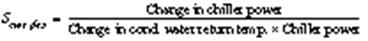 (25) (25)
If the chiller power increases by 2% for a 1°F increase in condenser water temperature, Scwr,des is equal to 0.02/°F. A large sensitivity factor means that the chiller power is very sensitive to the cooling tower control favoring operation at higher airflow rates (low PLRtwr,cap). The sensitivity factor should be evaluated at design conditions using chiller performance data. Typically, the sensitivity factor is between 0.01 and 0.03/°F. For multiple chillers with different performance characteristics, the sensitivity factor at design conditions is estimated as
Table 3 Parameter Estimates for Near-Optimal Tower Control Equation
Parameter |
One-Speed Fans |
Two-Speed Fans |
Variable-Speed Fans |
PLRtwr,cap |
PLR0 |
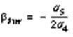
Ö2PLR0 |
Ö3PLR0 |
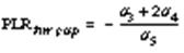
ßtwr |
1____ |
2____ |
1____ |
|
PLRtwr,cap |
3PLRtwr,cap |
2PLRtwr,cap |
Note: |
PLR0 = |
|
|
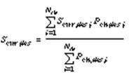 (26) (26)
where Scwr,des,i is the sensitivity factor and Pch,des,i is the power consumption for the ith chiller at the design conditions, and Nch is the total number of chillers.
The design approach to wet bulb atwr,des is the temperature difference between the condenser water supply and the ambient wet bulb for the tower, operating at its air and water flow capacity at plant design conditions. The design range rtwr,des is the water temperature difference across the tower at these same conditions (condenser water return minus supply temperature). The sum of atwr,des and rtwr,des is the temperature difference between the tower inlet and the ambient wet bulb and represents a measure of the tower’s capability to reject heat to ambient relative to the system requirements. A small temperature difference (tower approach plus range) results from a high tower heat transfer effectiveness or high water flow rate and yields lower condenser water temperatures with lower chiller power consumption. Typical values for the design approach and range are 7°F and 10°F.
The part-load ratio associated with the tower operating at full capacity, PLRtwr,cap may be greater than or less than one. Values less than unity imply that from an “energy point of view” the tower is not sized for optimal operation at design load conditions and that the tower should operate at its capacity for a range of loads less than the design load. Values of PLRtwr,cap greater than one imply that the tower is oversized for the design load and that the tower should never operate at its capacity.
For multiple chillers with very different performance characteristics, different open-loop parameters may be used for any combination of operating chillers. The sensitivity factors and chiller design power used to determine the open-loop control parameters in Table 3 should be estimated for each combination of operating chillers, and the part-load ratio used in Equation (23) should be determined using the design capacity for the operating chillers (not all chillers). In this case, Nch in Equation (26) represents the number of operating chillers.
Open-Loop Parameter Estimates Using Plant Measurements. Energy consumption can be reduced slightly by determining the open-loop control parameters from plant measurements. However, this results in additional complexity associated with implementation. One method for estimating the open-loop control parameters of Equation (23) from plant measurements involves performing a set of one-time trial-and-error experiments. At a given set of conditions (i.e., cooling load and ambient conditions), the optimal tower control is estimated by varying the fan settings and monitoring the total chiller and fan power consumption. Each tower control setting and load condition must be maintained for a sufficient time for the power consumption to approach steady-state and to hold the chilled-water supply temperature constant. The control setting that produces the minimum total power consumption is deemed optimal. This set of experiments is performed for a number of chilled-water cooling loads and the best-fit straight line through the resulting data points is used to estimate the parameters of Equation (23). As initial control settings for each load, Equation (23) may be used with estimates from design data as summarized in the previous section.
Another method for estimating the variables of Equation (23) uses an empirical model for total power consumption that is fit to plant measurements. The control that minimizes the power consumption associated with the model is then determined analytically. The section on Control Optimization Methods describes a general method for determining linear control relations in this manner using a quadratic model. For cooling tower fan control, chiller and fan power consumption are correlated with load and tower airflow for a constant chilled-water supply temperature using a quadratic function as follows:
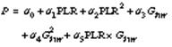 (27) (27)
where a0 to a5 are empirical constants determined through linear regression applied to measurements. For the quadratic function of Equation (27), the tower airflow that results in minimum power is a linear function of the PLR. The parameters of the open-loop control Equation (23) are then
 (28) (28)
 (29) (29)
For multiple chillers with very different performance characteristics, different open-loop parameters can be determined for any combination of operating chillers. In this case, separate correlations for near-optimal airflow or power consumption must be determined for each chiller combination.
Overrides for Equipment Constraints
The fractional tower airflow as determined by Equations (23) or (24) must be bounded between 0 and 1 according to the physical constraints of the equipment. Additional constraints on the temperature of the supply water to the chiller condensers are necessary to avoid potential chiller maintenance problems. Many (older) chillers have a low limit on the condenser water supply temperature that is necessary to avoid lubrication migration from the compressor. A high-temperature limit is also necessary to avoid excessively high pressures in the condenser, which can lead to compressor surge in centrifugal chillers. If the condenser water temperature falls below the low limit, then it is necessary to override the open-loop tower control and reduce the tower airflow to go above this limit. Similarly, if the high limit is exceeded, then the tower airflow should be increased as required.
Implementation
Before commissioning, the parameters of the open-loop control Equation (23) must be specified. These parameters are estimated using Table 3. After the system is in operation, these parameters may be fined-tuned with measurements as outlined previously. If multiple chillers have significantly different performance characteristics, it may be advantageous to determine different parameters for Equation (23) depending on the combination of operating chillers.
The relative tower airflow must be converted to a specific set of tower fan settings using the sequencing rules defined previously. This involves defining a relationship (i.e., table) for fan settings as a function of tower airflow. The table is constructed by defining the best fan settings for each possible increment of airflow. The conversion process between the continuous output of Equations (23) or (24) and the fan control involves choosing the set of discrete fan settings from the table that produces a lower airflow closest to the desired flow. However, in general, it is better to have greater rather than less than the optimal airflow. A good general rule is to choose the set of discrete fan controls that results in a relative airflow that is closest to, but not more than 10% less than, the output of Equations (23) or (24).
With the parameters of Equation (23) specified, the following procedure is applied at each decision interval (e.g., 15 min) to determine the tower control:
1. If the temperature of the supply water to the chiller condenser is less than the low limit, then reduce the tower airflow by one increment according to the near-optimal sequencing rules and exit the algorithm. Otherwise go to Step 2.
2. If the temperature of the supply water to the chiller condenser is greater than the high limit, then increase the tower airflow by one increment according to the near-optimal sequencing rules and exit the algorithm. Otherwise go to Step 3.
3. Determine the chilled-water load relative to the design load.
4. If the chilled-water load has changed by a significant amount (e.g., 10%) since the last control change, then go to Step 5. Otherwise exit the algorithm.
5. If the part-load ratio is greater than 0.25, then compute the near-optimal tower airflow as a fraction of the tower capacity, Gtwr, with Equation (23). Otherwise, determine Gtwr with Equation (24).
6. Limit Gtwr to keep the change from the previous decision interval less than a minimum value (e.g., less than 0.1 change).
7. Restrict the value of Gtwr between 0 and 1.
8. Convert the value of Gtwr to a specific set of control functions for each of the tower cell fans according to the near-optimal sequencing rules.
Implementation of this procedure requires some estimate of the chilled-water load, along with a measurement of the condenser water supply temperature. However, the accuracy of the load estimates is not extremely critical. In general, near-optimal control determined with load estimates that are accurate to within 5 to 10% results in total power consumption that is within 1% of the minimum. The best method for determining the chilled-water load is from the product of the measured chilled-water flow rate and the temperature difference between the chilled-water return and supply. For systems that use constant flow pumping to the chillers, the flow rates may be estimated from design data for the pumps and system pressure-drop characteristics.
Example 1. Consider an example plant consisting of four 550 ton chillers with four cooling tower cells, each having two-speed fans. Each chiller consumes approximately 330 kW at the design capacity, while each tower fan uses 40 kW at high speed. At design conditions, the chiller power increases approximately 6.6 kW for a 1°F increase in condenser water temperature, giving a sensitivity factor of 6.6/330 or 0.02/°F. The tower design approach and range from manufacturer’s data are 7 and 10°F.
Solution:
The first step in applying the open-loop control algorithm to this problem is the determination of the parameters of Equation (1) from the design data. From Table 3, the part-load ratio at which operation of the tower is at its capacity is estimated for the two-speed fans as
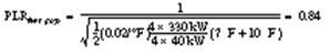
while the slope of the fractional airflow versus part-load ratio is estimated to be
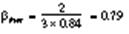
Given these parameters and the part-load ratio, the fractional tower airflow is estimated as
IF (PLR > 0.25) THEN
Gtwr = 1 – btwr (PLRtwr,cap – PLR)
ELSE
Gtwr = 4 PLR [1 – btwr (PLRtwr,cap – 0.25)]
Gtwr = MIN [1, MAX(0, Gtwr)]
To convert Gtwr into a specific tower control, the tower sequencing must be defined. The following table gives this information in a form that specifies the relationship between Gtwr and tower control for this example.
Cooling Tower Fan Sequencing for Example 1
|
Sequence No. |
Gtwr |
Tower Fan Speeds |
|
Cell #1 |
Cell #2 |
Cell #3 |
Cell #4 |
|
1 |
0.125 |
Low |
Off |
Off |
Off |
|
2 |
0.250 |
Low |
Low |
Off |
Off |
|
3 |
0.375 |
Low |
Low |
Low |
Off |
|
4 |
0.500 |
Low |
Low |
Low |
Low |
|
5 |
0.625 |
High |
Low |
Low |
Low |
|
6 |
0.750 |
High |
High |
Low |
Low |
|
7 |
0.875 |
High |
High |
High |
Low |
|
8 |
1.000 |
High |
High |
High |
High |
For a specific chilled-water load, the fan control should be the sequence of tower fan settings from the table that results in a value of Gtwr that is closest to, but not more than 10% less than, the output of Equations (1) or (2). Note that this example assumes that proper water flow can be maintained over all cooling tower cells.
Chilled-Water Reset With Fixed-Speed Pumping
Figure 25 shows a common configuration using fixed-speed chilled-water pumps with two-way valves at the cooling coils. A two-way bypass valve controlled to maintain a fixed pressure difference between the main supply and return lines is used to ensure relatively constant flow through chiller evaporators and reduce pressure drop and pumping costs at low loads. However, additional pump and chiller power savings can be realized by adjusting the chilled-water supply temperature to keep some cooling-coil valves open and thereby minimize the bypass flow.
Ideally, the chilled-water temperature should be adjusted to maintain all discharge air temperatures with a minimal number of cooling-coil control valves in a saturated (fully open) condition. The procedure described in this section is designed to accomplish this goal in a reliable and stable manner that reacts quickly to changing conditions.
(insert this Figure?)
Fig. 25 Typical Chilled-Water Distribution for Fixed-Speed Pumping
Pump Sequencing
Individual chilled-water pumps are commonly physically dedicated to individual chillers. In this case, the sequencing of chilled-water pumps is defined by the sequencing of chillers. In some installations, the chiller pumps are not dedicated to chillers, but instead are arranged in parallel, sharing common headers. In this case, the order for bringing pumps online and offline and the conditions for adding or removing chilled-water pump capacity must be specified. For pumps of different capacities, the logical order for bringing pumps online is from small to large. For pumps of similar capacity, the most efficient pumps should be brought online first and taken offline last.
Optimal Chilled-Water Temperature
One method for determining the optimal chilled-water temperature is to monitor the water control valve positions of “representative” air handlers and to adjust the set temperature incrementally at fixed decision intervals until a single control valve is fully open. The representative air handlers should be chosen to include load diversity at all times and ensure reliable data. One difficulty of this control approach is that valve position data are often unreliable. The valve could be stuck open or the saturation indicator could be faulty. This problem can be overcome by also monitoring discharge air temperatures, using them as a consistency check on valve position data. If a valve is unsaturated, this implies that the coil has sufficient capacity to maintain the discharge air temperature near the set point. Conversely, if a valve remains saturated at 100% open, the discharge air temperature should ultimately increase above the set point. These considerations lead to the following simple rules for increasing or decreasing the chilled-water set point in response to valve position and discharge air temperature data.
- If all water valves are unsaturated or the discharge air temperatures associated with all saturated valves are lower than the set point, increase the chilled-water set temperature.
- If more than one valve is saturated at 100% open and their corresponding discharge air temperatures are greater than their set points, decrease the chilled-water temperature.
In implementing these rules, a fixed increment for increasing or decreasing the chilled-water temperature must be chosen. A small increment results in more stable control, but also results in a slow response to sudden changes in load or supply air temperature set points. Using a first-order approximation, the chilled-water temperature can be reset in response to sudden changes in load and supply air temperature set point according to
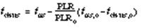 (30) (30)
where
tchws = new chilled-water set-point temperature
tas = current supply air set-point temperature
PLR = current part-load ratio (chiller load divided by total design load for all chillers)
tchws,o = chilled-water set point associated with last control decision
tas,o = supply air set point associated with last control decision
PLRo = part-load ratio associated with last control decision
Equation (30) assumes that the chilled-water temperature associated with the last control decision was optimal. As a result, it only applies to anticipating the effects of significant changes in the load and supply air set-point temperature on the optimal chilled-water set point. The “bump-and-wait” strategy fine-tunes the chilled-water supply temperature when the load and supply air set point are stable. For a variable air volume system, the supply air set points are most often constant and identical for all air-handling units. However, for a constant air volume system, these set points may vary with different air handlers. In this case, the supply air set point to use in Equation (30) should be an average value for the representative air handlers.
Equation (30) indicates that the optimal chilled-water supply temperature increases with increasing supply air temperature and decreasing load. This is because these changes cause the cooling-coil valves to close; optimal control involves keeping at least one valve open. Increasing supply air temperature causes the cooling-coil valves to close somewhat because of a larger average temperature difference for heat transfer between the water and air. A lower load requires smaller air-to-water temperature differences, which also leads to control valves closing.
Overrides for Equipment and Comfort Constraints
For a given chiller load, the chilled-water temperature has both upper and lower limits. The lower limit is necessary to avoid ice formation on the evaporator tubes of the chiller. This limit depends primarily on the load in relation to the size of the evaporator or, in other words, the temperature difference between the chilled water and refrigerant. At small temperature differences (large area or small load), the evaporator can tolerate a lower chilled-water temperature to avoid freezing than at large temperature differences. The lower limit on the chilled-water set point should be evaluated at the design load, because the overall system performance is improved by increasing chilled-water temperature above this limit for loads less than design. This lower limit can range from 38 to 44°F.
An upper limit on the chilled-water temperature arises from comfort constraints associated with the zones and the possibility of microbial growth associated with high humidities. For the available flows, the chilled-water temperature should be low enough to provide discharge air at a temperature and humidity sufficient to maintain all zones in the comfort region and avoid microbial growth. This upper limit varies with both load and entering air conditions and is accounted for by monitoring the zone conditions to ensure that they are in the comfort zone. If zone temperatures or humidities are not within reasonable bounds, then the discharge air temperature set point should be lowered.
Implementation
At each decision interval (e.g., 5 min), the following algorithm would be applied for determining the optimal chilled-water set-point temperature:
1. Determine the time-averaged total chilled-water load for the previous decision interval.
2. If the chilled-water load or supply air set-point temperature has changed by a significant amount (e.g., 10%) since the last control change, then estimate a new optimal chilled-water set point with Equation (30) and go to Step 6. Otherwise, go to Step 3.
3. Determine the time-averaged position of (or controller output for) the cooling-coil water valves and corresponding discharge air temperatures for representative air handlers.
4. If more than one valve is saturated at 100% open and their corresponding supply air temperatures are greater than set point (e.g., 1°F), then decrease the chilled-water temperature by a fixed amount (e.g., 0.5°F) and go to Step 6. Otherwise, go to Step 5.
5. If all water valves are unsaturated or the supply air temperatures associated with all valves that are saturated are lower than the set point, then raise the chilled-water set temperature by a fixed amount (e.g., 0.5°F). Otherwise, exit the algorithm with the chilled-water set point unchanged.
6. Limit the chilled-water set-point temperature between the upper and lower limits dictated by comfort, humidity, and equipment safety.
Implementing this algorithm requires some estimate of the chilled-water load, along with a measurement of the discharge air temperatures and control valve positions. However, a highly accurate estimate of the load is not necessary.
Chilled-Water Reset With Variable-Speed Pumping
Figure 26 shows a common configuration for systems using variable-speed chilled-water pumps with primary/secondary water loops. The primary pumps are fixed speed and are generally sequenced with chillers to provide a relatively constant flow of water through the chiller evaporators. The secondary chilled-water pumps are variable speed and are typically controlled to maintain a specified set point for pressure difference between supply and return flows for the cooling coils.
Although variable-speed pumps are usually used with primary/secondary chilled-water loops, they may also be applied to systems with a single chilled-water loop. In either case, variable-speed pumps offer the potential for a significant operating cost saving when both chilled-water and pressure differential set points are optimized in response to changing loads. This section presents an algorithm for determining near-optimal values of these control variables.
Optimal Differential Pressure Set Points
In practically all variable-speed chilled-water pumping applications, the pump speed is controlled to maintain a constant pressure differential between the main chilled-water supply and return lines. However, this approach is not optimal. To maintain a constant pressure differential with changing flow, the control valves for the air-handling units must close as the load (i.e., flow) is reduced, resulting in an increase in the flow resistance. The best strategy for a given chilled-water set point is to reset the differential pressure set point to maintain all discharge air temperatures with at least one control valve in a saturated (fully open) condition. This results in a relatively constant flow resistance and greater pump savings at low loads. With variable differential pressure set points, optimizing the chilled-water loop is described in terms of finding the chilled-water temperature that minimizes the sum of the chiller and pumping power, with the pump control dependent on the set point and the load.
Near-Optimal Chilled-Water Set Point
The optimal chilled-water supply temperature at a given load results from a tradeoff between chiller and pumping power, as illustrated in Figure 27. As the chilled-water temperature increases, the chiller power is reduced due to a reduction in the lift requirements of the chiller. For a higher set temperature, more chilled-water flow is necessary to meet the load requirements, and the pumping power requirements increase. The minimum total power occurs at a point where the rate of increase in pumping power with chilled-water temperature is equal to the rate of decrease in chiller power. This optimal set point moves to lower values as the load increases.
Braun et al. (1989a) demonstrated that the optimal chilled-water set point varies as a near-linear function of both load and wet-bulb temperature over a wide range of conditions. Figure 28 shows an example of how the optimal set point varies for a specific plant. The set point is plotted as a function of load relative to design load for two different wet-bulb temperatures. In general, the optimal chilled-water temperature decreases with load because the pump power becomes a larger fraction of the total power. A lower set point limit is set to avoid conditions that could form ice on evaporator tubes or too high a chiller “lift,” and an upper limit is established to ensure adequate cooling-coil dehumidification. For a given load, the chilled-water set point increases with wet-bulb temperature because the energy transfer across each cooling coil is proportional to the difference between its entering air wet-bulb temperature and the entering water temperature (the chilled-water set point). For a constant load, this temperature difference is constant and the chilled-water supply temperature increases linearly with entering air wet-bulb temperature.
The results of Figure 28 were obtained for a system where both the chilled-water supply and supply air set points to the zones were optimized. For this case, the supply air temperatures varied between 55°F at high loads and 60°F at low loads. More typically, supply air temperatures are constant at 55°F, and the variation in chilled-water supply temperature is smaller than that shown in Figure 27.
Figure 29 depicts the general form for an algorithm to determine chilled-water supply set points as a function of load and the average wet-bulb temperature entering the cooling coils. A normalized difference between the entering air wet-bulb temperature and the chilled-water supply temperature is shown as a linear function of the part-load ratio. The (unconstrained) chilled-water set point is determined as
tchws = tmx,wb – G(tmx,wb,des – tchws,des) (31)
where
G = 1 – bchws (PLRchws,cap – PLR) (32)
tchws = chilled-water supply temperature set point
tmx,wb = average or “representative” wet-bulb temperature of air entering cooling coils
tchws,des = chilled-water supply temperature at design conditions
tmx,wb,des = wet-bulb temperature of air entering cooling coils at design conditions
PLR = chilled-water load divided by the total chiller cooling capacity (part-load ratio)
PLRchws,cap = part-load ratio (value of PLR) at which G = 1
bchws = slope of the G versus part-load ratio (PLR) function
The result of Equation (31) must be constrained between upper and lower limits dictated by equipment safety (evaporator freezing), the machine operating envelope, and comfort and humidity concerns.
The variables of Equation (32) that yield near-optimal control depend on the characteristics of system. Detailed measurements over a range of conditions may be used to determine estimates of these parameters. However, this requires measuring component power consumption along with considerable time and expertise, and may not be cost effective unless performed by on-site plant personnel. Alternatively, simple estimates of these parameters may be obtained using design data.
Fig. 27 Tradeoff of Chiller and Pump Power with Chilled-Water Set Point
Open-Loop Parameter Estimates Using Design Data. Reasonable estimates of the parameters of Equation (32) may be determined analytically using design information as summarized in Table 4. These estimates were derived by applying optimization theory to a simplified mathematical model of the chiller and secondary-loop water pumps, assuming that a differential pressure reset strategy is used, pump efficiencies are constant, and the supply air temperature is not varied in response to changes in chilled-water supply temperature. In general, these parameter estimates are conservative in that they should provide a relatively low estimate of the optimal chilled-water set point.
Table 4 Parameter Estimates for Near-Optimal
Parameter |
Estimate |
PLRchws,cap |
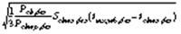
|
ßchws |

|
The design factors that affect the parameter estimates given in Table 4 are (1) the ratio of the chiller power to chilled-water pump power at design conditions Pch,des/Pchwp,des, (2) the sensitivity of the chiller power to changes in chilled-water temperature at design conditions Schws,des, and (3) the difference between the design entering air wet-bulb temperature to the cooling coil and the chilled-water supply temperature (tmx,wb,des – tchws,des).
The chiller power consumption at design conditions is the total power consumption of all plant chillers operating at their design cooling capacity. Likewise, the design pump power is the total power associated with all secondary chilled-water supply pumps operating at high speed. As the ratio of chiller power to pump power increases, it becomes more beneficial to operate the chillers at higher chilled-water temperatures and the pumps at higher flows. This is reflected in an increase in PLRchws,cap. If chiller power were free, then PLRchws,cap would go to zero, and the best strategy would be to operate the chillers at the minimum possible set point, resulting in low chilled-water flow rates. Typical values for the ratio of the chiller power to the pump power at design conditions are between 10 and 20, depending primarily on whether primary/secondary pumping is used.
The chiller sensitivity factor Schws,des is the incremental increase in chiller power for each degree decrease in chilled-water temperature as a fraction of the power:
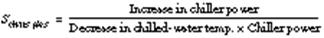 (33) (33)
If chiller power increases by 2% for a 1°F decrease in chilled-water temperature, then Schws,des is equal to 0.02/°F. A large sensitivity factor means that chiller power is very sensitive to the set point control favoring operation at higher set point temperatures and flows (higher PLRchws,cap). The sensitivity factor should be evaluated at design conditions using chiller performance data. Typically, the sensitivity factor is between 0.01 and 0.03/°F. For multiple chillers with different performance characteristics, the sensitivity factor at design conditions is estimated as
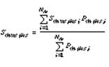 (34) (34)
where Schws,des,i is the sensitivity factor and Pch,des,i is the power consumption for the ith chiller at design conditions, and Nch is the total number of chillers.
The design difference between coil inlet air wet-bulb temperature and entering water temperature should be evaluated for a typical air handler operating at design load and flows. A small temperature difference results from a high coil heat transfer effectiveness or high water flow rate, allowing higher chilled-water temperatures with lower chiller power consumption. This is evident from Equation (31), where chilled-water set point decreases linearly with (tmx,wb,des – tchws,des) for a given G, and G is inversely related to the square root of (tmx,wb,des – tchws,des). Typically, this temperature difference is about 20°F.
Example 2. Consider an example plant with primary/secondary chilled-water pumping. There are four 550 ton chillers, each with a dedicated primary pump. Each chiller consumes approximately 330 kW at the design capacity. At design conditions, the chiller power increases approximately 6.6 kW for a 1°F decrease in chilled-water temperature, giving a sensitivity factor of 6.6/330 or 0.02/°F. The design chilled-water set point is 42°F, and the coil entering wet-bulb temperature is 62°F at design conditions. The secondary loop uses three identical 60 hp chilled-water pumps: one with a variable-speed and two with fixed-speed motors.
Solution:
The first step in applying the open-loop control algorithm to this problem is the determination of the parameters of Equation (10) from the design data. From Table 4, the part-load ratio at which the chilled-water temperature reaches a minimum (with the design entering wet-bulb temperature to the coils) is
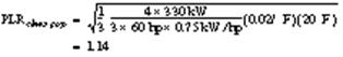
and the slope of the set point versus part-load ratio is estimated to be
Given these parameters and the part-load ratio, the unconstrained chilled-water set-point temperature from Equations (31) and (32) is then
tchws = tmx,wb – [1 – 0.44(1.14 – PLR)]20
Pump Sequencing
Variable-speed pumps are sometimes used in combination with fixed-speed or other variable-speed pumps. Pump sequencing involves determining both the order and point that pumps should be brought online and offline.
Pumps should be brought online in an order that allows a continuous variation in flow rate and maximized operating efficiency of the pumps at each switch point for the specific pressure loss characteristic. For a combination of fixed-speed and variable-speed pumps, at least one variable-speed pump should be brought online before any fixed-speed pumps. For single-loop systems (i.e., no secondary loop) with variable-speed pumps, the pressure-drop characteristics change when chillers are added or removed and the optimal sequencing of pumps depends on the sequencing of chillers.
An additional pump should be brought online whenever the current set of pumps is operating at full capacity and can no longer satisfy the differential pressure set point. This situation can be detected by monitoring the differential pressure or the controller output signal. Insufficient pump capacity leads to extended periods with differential pressures that are less than the set point and a controller output that is saturated at 100%. A pump may be taken offline whenever the remaining pumps have sufficient capacity to maintain the differential pressure set point. This condition can be determined by comparing the current (time-averaged) controller output with the controller output (time-averaged) at the point just after the last pump was brought online. The pump can be brought offline when the current output is less than the switch point value by a specified dead band (e.g., 5%).
Overrides for Equipment and Comfort Constraints
The chilled-water temperature is bounded by upper and lower limits dictated by comfort, humidity, and equipment safety concerns. However, within these bounds, the chilled-water temperature may not always be low enough to maintain supply air set-point temperatures for the cooling coils. This situation might occur at high loads when the chilled-water flow is at a maximum and is detectable by monitoring the coil discharge air temperatures. Limits on the pressure differential set point might also be imposed to ensure adequate controllability of the cooling-coil control valves.
Implementation
Before commissioning, the parameters of the open-loop control for chilled-water set point [Equation (32)] need to be estimated using the results of Table 4. After the system is in operation, these parameters may be fine-tuned with measurements as outlined in the section on Control Optimization Methods. With the parameters specified, the control algorithm is separated into two reset strategies: chilled-water temperature and pressure differential.
Chilled-Water Temperature Reset. The chilled-water supply temperature set point is reset at fixed decision intervals (e.g., 15 min) using the following procedure:
1. Determine the time-averaged position of (or controller output for) the cooling-coil water valves and corresponding discharge air temperatures for “representative” air handlers over the previous decision interval.
2. If more than one valve is saturated at 100% open and their corresponding discharge air temperatures are greater than set point (e.g., 1°F), then decrease the chilled-water temperature by a fixed amount (e.g., 0.5°F) and go to Step 5. Otherwise, go to Step 3.
3. Determine the total chilled-water flow and load.
4. Estimate an optimal chilled-water set point with Equations (9) and (10). Increase or decrease the actual set point in the direction of the near-optimal value by a fixed amount (e.g., 1°F).
5. Limit the new set point between upper and lower constraints dictated by comfort and equipment safety.
Pump Sequencing. Secondary pumps should be brought online or offline at fixed decision intervals (e.g., 15 min) with the following logic:
1. Evaluate the time-averaged pump controller output over the previous decision interval.
2. If the pump controller is saturated at 100%, then bring the next pump online. Otherwise, go to Step 3.
3. If the pump control output is significantly less (e.g., 5%) than the value associated with the first time interval after the last pump was brought online, then bring that pump offline.
Differential Pressure Reset. The set point for differential pressure between supply and return lines should be reset at smaller time intervals than the supply water temperature reset and pump sequencing strategies (e.g., 5 min) using the following procedure:
1. Check the water valve positions (or controller output) for “representative” air handlers and determine the time-averaged values over the last decision interval.
2. If more than one valve has been saturated at 100% open, then increase the differential pressure set point by a fixed value (e.g., 5% of the design value) and go to Step 4. Otherwise, go to Step 3.
3. If none of the valves have been saturated, then decrease the differential pressure set point by a fixed value (e.g., 5% of the design value).
4. Limit the differential pressure set point between upper and lower constraints.
Sequencing and Loading of Multiple Chillers
Multiple chillers are normally configured in parallel and typically controlled to give identical chilled-water supply temperatures. In most cases, controlling for identical set temperatures is the best and simplest strategy. With this approach, the relative loading on operating chillers is controlled by the relative chilled-water flow rates. Typically, the distribution of flow rates to heat exchangers for both chilled and condenser water are dictated by chiller pressure-drop characteristics and may be adjusted through flow balancing, but are not controlled using a feedback controller. In addition to the distribution of chilled and condenser water flow rates, the chiller sequencing affects energy consumption. Chiller sequencing defines the conditions under which chillers are brought online and offline. Simple guidelines may be established for each of these controls to provide near-optimal operation.
Near-Optimal Condenser Water Flow Distribution
In general, the condenser water flow to each chiller should be set to give identical leaving condenser water temperatures. This condition approximately corresponds to relative condenser flow rates equal to the relative loads on the chillers, even if the chillers are loaded unevenly. Figure 30 shows results for four sets of two chillers operated in parallel. The curves represent data from chillers at three different installations: (1) a 5500 ton variable-speed chiller at the Dallas-Ft. Worth Airport, Texas (Braun et al. 1989a); (2) a 550 ton fixed-speed chiller at an office building in Atlanta (Hackner et al. 1984, 1985); and (3) a 1250 ton fixed-speed chiller at a large office building in Charlotte, North Carolina (Lau et al. 1985). The capacities of the chillers in the two office buildings were scaled up for comparison with the Dallas-Ft. Worth airport chiller.
The overall chiller coefficient of performance (COP) is plotted versus the difference between the condenser water return temperatures for equal chiller loading. For multiple chillers having similar performance characteristics (either variable- or fixed-speed), it is best to distribute the condenser water flow rates so that each chiller has the same leaving condenser water temperature. For situations where chillers do not have identical performance, equal leaving condenser water temperatures result in chiller performance that is close to the optimum. Even for variable- and fixed-speed chiller combinations that have very different performance characteristics, the penalty associated with the use of identical condenser leaving-water temperatures is small. To achieve equal condenser leaving-water temperatures, it is necessary to properly balance the condenser water flow rates at design operating conditions.
Optimal Chiller Load Distribution
Assuming identical chilled-water return and chiller supply temperatures, the relative chilled-water load for each parallel chiller (load divided by total load) that is operating could be controlled by its relative chilled-water flow rate (flow divided by total flow). To change the relative loadings in response to operating conditions, the individual flow rates must be controlled. However, this is typically not done and it is probably sufficient to establish the load distributions based on design information and then balance the flow rates to achieve these load distributions. Alternatively, the individual chiller loads can be precisely controlled through variation of individual chiller supply water set points.
Chillers with Similar Performance Characteristics. Braun et al. (1989a) showed that for chillers with identical design COPs and part-load characteristics, a minimum or maximum power consumption occurs when each chiller is loaded according to the ratio of its capacity to the total capacity of all operating chillers. This is equivalent to each chiller operating at equal part-load ratios (load divided by cooling capacity at design conditions). For the ith chiller, the optimal chiller loading is then
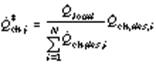 (35) (35)
where Qload is the total chiller load, Qch,des,i is the cooling capacity of the ith chiller at design conditions, and N is the number of chillers operating.
The loading determined with Equation (35) could result in either minimum or maximum power consumption. However, this solution gives a minimum when the chillers are operating at loads greater than the point at which the maximum COP occurs (i.e., chiller COP decreases with increased loading). Typically, the maximum COP occurs at loads that are less than the nominal design capacity.
Figure 31 shows the effect of relative loading on chiller COP for different sets of identical chillers loaded at approximately 70% of their total capacities. Three of the chiller sets have maximum COPs when evenly loaded [matching the criterion of Equation (35)], whereas the fourth (Dallas-Ft. Worth fixed-speed) obtains a minimum at that point. The part-load characteristic of the Dallas-Ft. Worth fixed-speed chiller is unusual in that the maximum overall COP occurs at its maximum capacity. This chiller was retrofitted with a different refrigerant and drive motor, which derated its capacity from 8700 to 5500 tons. As a result, the evaporators and condensers are oversized for its current capacity. Overall, the penalty associated with equally loading the Dallas-Ft. Worth fixed-speed chillers is small compared with optimal loading, and this strategy is probably appropriate. However, a slight reduction in energy consumption is possible if one of the two chillers operates at full capacity. The loading criterion of Equation (35) also works well for many combinations of chillers with different performance characteristics.
To achieve specified relative chiller loadings with equal chilled-water set points, chilled-water flow rates must be properly balanced. The relative loadings of Equation (35) only depend on design information, and flow balancing can be achieved through proper design and commissioning.
Chillers with Different Performance Characteristics. For the general case of chillers with significantly different part-load characteristics, a point of minimum or maximum overall power occurs where the partial derivatives of the individual chiller’s power consumption with respect to their loads are equal:
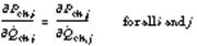 (36) (36)
and subject to the constraint that
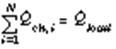 (37) (37)
where Qch,i is the cooling load for the ith chiller and Qload is the total cooling load.
In general, the power consumption of a chiller can be correlated as a quadratic function of cooling load and difference between the leaving condenser water and chilled-water supply temperatures according to
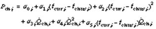 (38) (38)
where, for the ith chiller, tcwr is the leaving condenser water temperature and tchws is the chilled-water supply temperature. The coefficients of Equation (38) (a0,i to a5,i) can be determined for each chiller through regression applied to measured or manufacturers’ data.
If each chiller has identical leaving condenser and chilled-water supply temperatures, the criterion of Equation (36) applied to the correlation of Equation (38) leads to
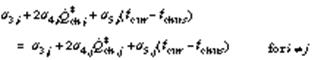 (39) (39)
where Q*ch,i is the optimal load for the ith chiller.
Equations (39) and (37) represent a system of N linear equations in terms of N chiller loads that can be solved to give minimum (or possibly maximum) power consumption. For a given combination of chillers, the solution depends on the operating temperatures and total load. However, the individual chiller loads must be constrained to be less than the maximum chiller capacity at these conditions. If an individual chiller load determined from these equations is greater than its cooling capacity, then this chiller should be fully loaded and Equations (39) and (37) should be resolved for the remaining chillers [Equation (39) should only include unconstrained chillers].
To control individual chiller loads with identical chilled-water supply temperatures, individual chilled-water flow rates need to be controlled with two-way valves, which is not typical. However, the distribution of chiller loads could be changed for a fixed-flow distribution by using different chilled-water set-point temperatures. For a given flow and load distribution, the individual chiller set point for parallel chillers is determined according to
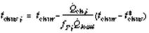 (40) (40)
where fF,i is the flow for the ith chiller divided by the total flow, t*chws is the chilled-water supply temperature set point for the combination of chillers determined using the previously defined reset strategies, and tchwr is the temperature of the water returned to the chillers from the building.
Substituting Equation (40) into Equation (38) and then applying the criterion of Equation (36) leads
Optimal chiller loads are determined by solving the linear system of equations represented by Equations (41) and (37). The individual chiller set points are then evaluated with Equation (40). If any set points are less than the minimum set point or greater than the maximum set point, then the set point should be constrained and Equations (41) and (37) should be resolved for the remaining chillers [Equation (41) should only include unconstrained chillers].
Example 3. Determine the optimal loading for two chillers using the three methods outlined in this section. Table 5 gives the design cooling capacities and coefficients of the curve-fit of Equation (38) for the two chillers. The chillers are operating with a total cooling load of 1440 tons, condenser water return temperature of 85°F, an overall chilled-water supply temperature set point of 45°F, and a chilled-water return temperature of 55°F. Figure 32 shows the COPs for the two chillers as a function load relative to their design loads for the given operating temperatures. Chiller 1 is more efficient at higher part-ratios and less efficient at lower part-load ratios as compared with Chiller 2.
Solution:
First, consider operating the chillers at equal part-load ratios. The ratio of the cooling load to the cooling capacity of the operating chillers is 1440/(1250 + 550) = 0.85. From Equation (35), the individual chiller loads are
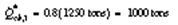
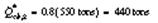
The power for each chiller is computed for the specified operating conditions with Equation (38) and the coefficients of Table 5. For the case of equal part-load ratios, the total chiller power consumption is

A second solution is determined for optimal chiller loads for the case of equal chilled-water temperature set points and controllable flow for each chiller. In this case, algebraic manipulation of Equations (37) and (39) produces the following results for the individual chiller loads:
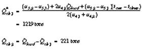
The resulting power consumption is then

Optimal loading of the chillers reduces the overall chiller power consumption by about 4% through heavier loading of Chiller 1 and lighter loading of Chiller 2 (see Figure 32).
Finally, optimal chiller loading is determined for the case where the individual loadings are controlled by using different chilled-water temperature set points (individual flow is not controllable). To apply Equations (40) and (41), the relative chilled-water flow rate for each chiller must be known. For this example, the relative flow for the ith chiller is assumed to be equal to the ratio of its design capacity to the design capacity for the operating chillers, so that
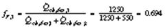
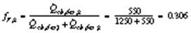
Then, solving Equations (37) and (41) leads to the following results for the individual chiller loads:
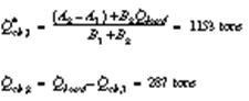
These loads lead to a total chiller power consumption of

Individual chilled-water set points are determined from Equation (40) and are 43.5 and 48.5°F for Chillers 1 and 2, respectively. Power consumption has increased slightly from the case of identical chiller set points and variable flow.
Note that changing either flows or chilled-water set points complicates overall system control as compared with loading the chillers with fixed part-load ratios, and leads to relatively small savings.
Table 5 Chiller Characteristics for Optimal Loading Example 3
Variable |
Units |
Chiller 1 |
Chiller 2 |
Q·ch,des,i |
tons |
1250 |
550 |
a0,i |
kW |
106.4 |
119.7 |
a1,i |
kW/°F |
6.147 |
0.1875 |
a2,i |
kW/°F2 |
0.1792 |
0.04789 |
a3,i |
kW/ton |
–0.0735 |
–0.3673 |
a4,i |
kW/ton2 |
0.0001324 |
0.0005324 |
a5,i |
kW/ton·°F |
–0.001009 |
0.008526 |
Order for Bringing Chillers Online and Offline
For chillers with similar efficiencies, the order in which chillers are brought online and offline may be dictated by their cooling capacities and the desire to provide even runtimes. However, whenever beneficial and possible, chillers should be brought online in an order that minimizes the incremental increase in energy consumption. At a given condition, the power consumption of any chiller can be evaluated using the correlation given by Equation (38), where the coefficients are determined using manufacturers’ data or in-situ measurements. Then, the overall power consumption for all operating chillers is
 (42) (42)
When additional chiller capacity is required (see next section), the projected power of all valid chiller combinations should be evaluated using Equation (38), with the projected load determined by Equation (35) for chillers with similar performance characteristics, or the solution of Equations (36) subject to the constraint in Equation (37) for chillers with significantly different performance characteristics. Valid chiller combinations involve chillers that are not in alarm or locked out, and with load ratios between a low limit (e.g., 30%) and 100%. The best chiller combination to bring on line should result in the smallest increase (or largest decrease) in overall chiller power consumption as estimated with Equations (42) and (38) with chiller loading determined as outlined in the previous section. For systems with dedicated chilled-water and condenser water pumps and/or cooling towers, the associated power of this equipment should be added to Equation (38) to estimate the load of the chiller plus its auxiliary equipment. It is recommended that these estimates be performed online using in-situ measurements of each chiller’s discharge chilled-water temperature and entering condenser water temperature, and the projected load of the chiller. A chiller should be shut down when its load drops below the spare capacity load of the current number of online chillers; for a primary/secondary chilled-water system, the primary chilled-water flow will remain above the secondary chilled-water flow once the chiller is shut down. (The spare capacity load is equal to the rated capacity of the online chillers minus the actual measured load of the online chillers.)
For chillers with similar design cooling capacities, a simpler (although suboptimal) approach can be used for determining the order for bringing chillers online and offline. In this case, the chiller with the highest peak COP can be brought online first, followed by the second most efficient chiller, etc., and then brought offline in reverse order. The maximum COP for each chiller can be evaluated using manufacturers’ design and part-load data or from curve-fits to in-situ performance.
The chiller load associated with maximum COP for each chiller can be determined by applying a first-order condition for a maximum, using Equation (38) and the definition of COP. For this functional form, the maximum (or possibly minimum) COP occurs for
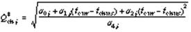 (43) (43)
The load determined from Equation (43) yields a maximum COP whenever it is real and bounded between upper and lower limits. Otherwise, it can be assumed that the maximum COP occurs at full load conditions. Typically, the maximum COP occurs between about 40 and 80% of design load and increases as the temperature difference between the condenser leaving water and chilled-water supply decreases. Equation (43) could be applied online to determine the rank ordering of chillers to bring online as a function of operating temperatures. However, it is often sufficient to use Equation (43) at the design temperature difference and establish a chiller sequencing order at the design or commissioning stage.
Example 4. Determine the loads for maximum COP for two different chillers at a chilled-water set point of 45°F and a condenser water return temperature of 80°F. Table 6 gives the design cooling capacities and coefficients of the curve-fit of Equation (38) for the two chillers. Figure 33 shows the COPs of the two chillers determined from the correlations as a function of relative load (PLR) and temperature difference (tcwr – tchws). These chillers have identical performance at design conditions, but very different part-load characteristics because of different methods used for capacity control.
Solution:
The loading associated with the maximum COP for each chiller is determined using Equation (43) and the coefficients of Table 6. The power for each chiller is then determined using Equation (38) and the COP follows directly. Results of the calculations are given in Table 7. The maximum COP for chiller A is about 20% greater than that for chiller B at the specified operating temperatures and should be brought online first.
Table 6 Chiller Characteristics for Maximum COP, Example 4
Variable |
Unit |
Chiller A |
Chiller B |
Q·ch,des,i |
tons |
5421 |
5421 |
a0,i |
kW |
262.6 |
187.2 |
a1,i |
kW/°F |
–25.36 |
96.19 |
a2,i |
kW/°F2 |
0.9718 |
–0.4314 |
a3,i |
kW/ton |
–0.02568 |
–0.4314 |
a4,i |
kW/ton2 |
0.00004046 |
0.0001106 |
a5,i |
kW/ton·°F |
0.005289 |
–0.004537 |
Table 7 Results for Maximum COP, Example 4
Variable |
Chiller A |
Chiller B |
Q·*ch,i |
3738 ton |
5229 ton |
PLRi |
0.690 |
0.965 |
Pch,i |
1727 kW |
2964 kW |
COPi |
7.61 |
6.21 |
Load Conditions for Bringing Chillers Online or Offline
In general, chillers should be brought online at conditions where the total power (including pumps and tower or condenser fans) of operating with the additional chiller would be less than without it. Conversely, a chiller should be taken offline when the total power of operating with that chiller would be less than with it. In practice, the switch point for bringing a chiller online should be greater than that for bringing that same chiller offline (e.g., 10%), to ensure a stable control. The optimal sequencing of chillers depends primarily on their part-load characteristics and the manner with which the chiller pumps are controlled.
Dedicated Pumps. Where individual condenser and chilled-water pumps are dedicated to the chiller, Hackner et al. (1985) and Braun et al. (1989a) showed that a chiller should be brought online when the operating chillers reach their capacity. This conclusion is the result of considering both the chiller and pumping power in determining optimal control. If pumping power is ignored, the optimal chiller sequencing occurs when chiller efficiency is maximized at each load. Because maximum efficiency often occurs at part-load conditions, the optimal point for adding or removing chillers may occur when chillers are operating at less than their capacity. However, the additional pumping power required for bringing additional pumps online with the chiller offsets any reductions in overall chiller power consumption associated with part-load operation.
When pumps are dedicated to chillers, situations may arise where chillers are operating at less than their capacity but chilled-water flow to the cooling coils is insufficient to meet the building load. This generally results from inadequate design or improper maintenance. Under these circumstances, either some zone conditions need to float to reduce the chilled-water set point (if possible), or an additional chiller needs to be brought online. Monitoring the zone air-handler conditions is one way to detect this situation. If (1) the chilled-water set point is at its lower limit, (2) any air-handler water control valves are saturated at 100% open, and (3) their corresponding discharge air temperatures are significantly greater (e.g., 2°F) than set point, then the chilled-water flow is probably insufficient and an additional chiller/pump combination could be brought online. One advantage of this approach is that it is consistent with the reset strategies for both fixed- and variable-speed chilled-water systems.
Chillers can be brought online or offline with the following logic:
1. Evaluate the time-averaged values of the chilled-water supply temperature and overall cooling load over a fixed time interval (e.g., 5 min).
2. If the chilled-water supply temperature is significantly greater than the set point (e.g., 1°F), then bring the next chiller online. Otherwise, go to Step 3.
3. Determine the time-averaged position of the cooling-coil water valves and corresponding discharge air temperatures for “representative” air handlers.
4. If the chilled-water supply set point is at its lower limit and more than one valve is saturated at 100% open and their corresponding discharge air temperatures are significantly greater than set point (e.g., 1°F), then bring another chiller/pump combination online. Otherwise, go to Step 5.
5. If the cooling load is significantly less (e.g., 10%) than the value associated with the first time interval after the last chiller was brought online, then take that chiller offline.
Nondedicated Pumps. For systems without dedicated chiller pumps (e.g., variable-speed primary systems), the optimal load conditions for bringing chillers online or offline do not generally occur at the full capacity of the chillers. In determining optimal chiller switch points, ideally both chiller and pumping power should be considered because pressure-drop characteristics and pumping change when a chiller is brought online or offline. However, simple estimates of optimal switch points may be determined by considering only the chiller power.
A chiller should be brought online whenever it would reduce the overall chiller power or if the current chillers can no longer meet the load (see previous section). A chiller should be added if the power consumption associated with (N + 1) chillers is significantly less (e.g., 5%) than the current N chillers, with both conditions evaluated using Equation (20) with correlations of the form given in Equation (38), and sequencing and loading determined as outlined in previous sections. Conversely, a chiller should be removed if the power consumption associated with the (N – 1) chillers is significantly less (e.g., 5%) than the current N chillers. The decision to add or remove chillers is readily determined using the current load and operating temperatures.
Strategies for Boilers
Load Conditions for Bringing Boilers Online or Offline
The specifics of the strategy for bringing boilers online depend on the type of boiler. Hot-water boilers have dedicated or nondedicated hot-water pumps; steam boilers do not have hot-water pumps, but rely on differences in steam pressure between the boiler steam header discharge and the point of use to distribute steam throughout the system.
Hot-water boilers with dedicated pumps. The strategy for hot-water boilers with dedicated hot-water pumps is similar to that for chillers with dedicated chilled-water and condenser water pumps: another boiler should be brought online when operating boilers reach capacity, because the efficiency of the boiler should include the power to drive its associated hot-water pump. This can be determined when hot-water temperature drops below its set point for a predetermined time interval (e.g., 5 min).
Hot-water boilers with dedicated pumps can be brought online and offline with the following logic:
1. Continuously calculate the load ratio of each boiler or boiler combination. For the ith boiler,
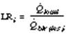 (44) (44)
where LRi is load ratio of the ith boiler combination, is the total boiler plant load, and is the design (rated) output of the ith boiler combination.
2. Every sampling interval (e.g., 60 s), calculate the predicted input fuel requirement for each boiler combination as
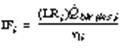 (45) (45)
where IFi is the input fuel requirement and hi is the efficiency of the ith boiler combination.
3. Continuously evaluate time-averaged values of the hot-water supply temperature over a fixed time interval (e.g., 5 min).
4. If the hot-water supply temperature drops below its set point for a predetermined time interval (e.g., 5 min), then, from boiler part-load performance curves, select the boiler combination with a load ratio between 0.5 and 1.0 and with the least input fuel requirement to meet the load, and turn this combination of boilers on. Note that this strategy will greatly reduce the possibility of short-cycling boilers because the new combination of boilers to be started will likely include boilers already operating (i.e., only one additional boiler is likely to be added).
5. If the capacity of the least efficient online boiler drops below the spare capacity of the current number of boilers operating (or for a primary-secondary hot-water system, if the flow rate of the associated primary hot-water pump is less than the difference between primary and secondary hot-water flow rates) for a predetermined time interval (e.g., 5 min), then shut down and bank this boiler in hot standby.
Hot-water boilers with nondedicated pumps or steam boilers. For hot-water systems without dedicated hot-water pumps or for steam systems, the optimal load conditions for bringing boilers online or offline do not generally occur at the full capacity of the online boilers. For these systems, a new boiler combination should be brought online whenever the hot-water supply temperature or steam pressure falls below set point for a predetermined time interval (e.g., 5 min) and the part-load efficiency curves of the boiler combination predicts that the new combination of boilers can meet the required load using significantly less (e.g., 5%) input fuel.
Optimal Boiler Load Distribution
Optimal load distribution strategies for boilers are similar to those for chillers. For boilers with similar performance characteristics, the optimal boiler loading is similar to Equation (35) for chillers:
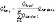 (46) (46)
where Q*blr,i is the optimal load for the ith boiler.
For boilers with significantly different performance characteristics, the criterion for optimal boiler loading is similar to Equations (36) and (37) for chillers, except that boiler cost of operation is used:
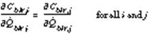 (47) (47)
and subject to the constraint that
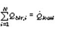 (48) (48)
where Cblr,i and Cblr, j are the operating costs of boiler i and j, respectively, is the heating load for the ith boiler, and Qload is the total heating load.
In general, the boiler operating-cost curve can be calculated as a quadratic function of heating load only. For the ith boiler,
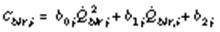 (49) (49)
Applying the criterion of Equation (47) to Equation (49),
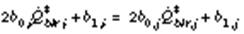 (50) (50)
where Q*blr,i is the optimal load for the ith boiler.
Maintaining Boilers in Standby Mode
It is generally more economical to run fewer boilers at a high rating. However, the integrity of the steam or hot-water supply must be maintained in the event of a forced outage of one of the operating boilers or if the facility experiences highly diverse load swings throughout the heating season. Both conditions can often be satisfied by maintaining a boiler in standby or “live bank” mode. For example, in this mode, a steam boiler is isolated from the steam system at no load but is kept at system operating pressure by periodic firing of either the igniters or a main burner to counteract ambient heat losses.
Supply Water and Supply Pressure Reset for Boilers
Simple control strategies can be used to generate a suboptimal hot-water temperature (for hot-water boilers) or steam pressure (for steam boilers). An energy management and control system must be interfaced to the boiler controls and be capable of monitoring the position of the valve controlling the flow of hot water to the heating coils or steam pressure at the most critical zone. For a hot-water system:
1. Continuously monitor the hot-water valve position of the various heating zones.
2. If none of the hot-water valves are greater than 95% open, lower the boiler hot-water supply temperature by a small increment (e.g., 1°F) each reset time interval (a predetermined interval established by system thermal lag characteristics, e.g., 15 to 20 min).
3. Once one hot-water valve opens beyond 95%, stop the downward resets of boiler hot-water temperature set point.
4. If two or more hot-water valves open beyond 95%, raise the boiler hot-water temperature set point by a small increment (e.g., 1°F) each reset interval.
For a steam system, the steam header pressure should be lowered to a value that just satisfies the highest pressure demand. Caution: for nongravity condensate return systems, steam pressure reset could impede condensate return (see Chapter 10, Steam Systems, of the 2004 ASHRAE Handbook—HVAC Systems and Equipment).
Strategies for Air-Handling Units
Air Handler Sequencing and Economizer Cooling
Traditional air-handler sequencing strategies use a single PI controller to control heating, cooling with outdoor air, mechanical cooling with 100% outdoor air, and mechanical cooling with minimum outdoor air. Sequencing between these different modes is accomplished by splitting the controller output into different regions of operation as shown in Figure 34.
Figure 34 depicts the relationship between the control signal to the valves and dampers and the feedback controller output. The controller adjusts its output to maintain the supply air temperature set point. If the output is between 100 and 200%, mechanical cooling is used. When outdoor conditions are suitable, the outdoor air dampers switch from minimum position (minimum ventilation air) to fully open. For a dry-bulb economizer, this switch point occurs when ambient air is less than a specified value. This switch point should be less than the switch point to return to minimum outdoor air, to ensure stable control. The economizer switchover temperature may be significantly lower than the return air temperature (e.g., 10°F lower) in humid climates where latent ventilation loads are significant. However, in dry climates, the switchover temperature may be close to the return temperature (e.g., 75°F). An enthalpy (or wet-bulb) economizer compares the outdoor and return air enthalpies (or wet-bulb temperatures) to initiate or terminate economizer operation. In general, enthalpy economizers yield lower energy costs than dry-bulb economizers, but require measurements of the outdoor and return air humidity. Humidity sensors require regular maintenance to ensure accurate readings. When controller output is between 0 and 100% (see Figure 34), the cooling-coil valve is fully closed and cooling is provided by ambient air only. In this case, the controller output modulates the position of the outdoor air dampers to maintain the set point. If the controller output signal is between –100 and 0%, the heating coil is used to maintain set point and the outdoor air dampers are set at their minimum position.
A single feedback controller is difficult to tune to perform well for all four modes of operation associated with an AHU. An alternative to the traditional sequencing strategy is to use three separate feedback controllers as described by Seem et al. (1999). This approach can improve temperature control, reduce actuator usage, and reduce energy costs. Figure 35 shows a state transition diagram for implementing a sequencing strategy that incorporates separate feedback controllers.
In State 1, a feedback controller adjusts the heating valve to maintain the supply air set-point temperature with minimum outdoor air. The transition to State 2 occurs after the control signal has been saturated at the no-heating position for a period equal to a specified state transition delay (e.g., 3 min). In State 2, a second feedback controller adjusts the outdoor and return air dampers to achieve set point with heating and cooling valves closed. Transition back to State 1 only occurs after the damper control signal is saturated at its minimum value for the state transition delay, whereas transition to State 3 is associated with saturation at the maximum damper position for the state transition delay. In State 3, the outdoor air damper remains fully open and a third feedback controller is used to adjust the flow of cooling water to maintain the supply air temperature at set point. Transition back to State 2 occurs if the controller output is saturated at its minimum value for the state transition delay. For a dry-bulb economizer, transition to State 4 occurs when the ambient dry-bulb temperature is greater than the switchover temperature by a dead band (e.g., 2°F). The feedback controller continues to modulate the cooling-coil valve to achieve set point. Transition back to State 3 occurs when the ambient dry-bulb is less than the switchover temperature (e.g., 65°F). For an enthalpy economizer, the ambient enthalpy is compared with return air enthalpy to initiate transitions between States 3 and 4.
Supply Air Temperature Reset for Constant Air Volume (CAV)
The benefits of resetting supply air temperature set points for CAV systems are significant. Increasing the supply air set point for cooling reduces both the cooling and reheat required, but does not change fan energy. In general, the set point for a CAV system could be set at the highest value that will keep all zone temperatures at their set points and all humidities within acceptable limits. A simple reset strategy based on this concept follows.
At each the decision interval (e.g., 5 min), the following logic can be applied:
1. Check the controller outputs for representative zone reheat units and determine time-averaged values over the last decision interval.
2. If any controller output is less than a threshold value (e.g., 5%), then decrease the supply air set point by a fixed value (e.g., 0.5°F) and go to Step 4. Otherwise, go to Step 3.
3. If all zone humidities are acceptable and all controller outputs are greater than a threshold value (e.g., 10%), then increase the discharge air set point by a fixed value (e.g., 0.5°F) and go to Step 4. Otherwise, do not change the set point.
4. Limit the set point between upper and lower limits based on comfort considerations.
Static Pressure Reset for Variable Air Volume (VAV)
Flow may be modulated in a VAV system by using dampers on the outlet side of the fan, inlet vanes on the fan, vane-axial fans with controllable pitch fan blades, or variable-speed control of the fan motor. Typically, the inputs to any of these controlled devices are modulated to maintain a duct static pressure set point as described in Chapter 46. In a single-duct VAV system, the duct static pressure set point is typically selected by the designer to be a fixed value. The sensor is located at a point in the ductwork such that the established set point will ensure proper operation of the zone VAV boxes under varying load (supply airflow) conditions. A shortcoming of this approach is that static pressure is controlled based on a single sensor intended to represent the pressure available to all VAV boxes. Poor location or malfunction of this sensor will cause operating problems.
For a fixed static pressure set point, all of the VAV boxes tend to close as zone loads and flow requirements decrease. Therefore, flow resistance increases with decreasing load. Significant fan energy savings are possible if the static pressure set point is reset so that at least one of the VAV boxes remains open. With this approach, flow resistance remains relatively constant. Englander and Norford (1992), Hartman (1993), Warren and Norford (1993), Wei et al. (2004) proposed several different strategies based on this concept. Englander and Norford used simulations to show that either static pressure or fan speed can be controlled directly using a flow error signal from one or more zones and simple rules. Their technique forms the basis of the following reset strategy.
At each decision interval (e.g., 5 min), the following logic can be applied:
1. Check the controller outputs for representative VAV boxes and determine time-averaged values over the last decision interval.
2. If any of the controller outputs are greater than a threshold value (e.g., 98%), then increase the static pressure set point by a fixed value (e.g., 5% of the design range) and go to Step 4. Otherwise, go to Step 3.
3. If all of the controller outputs are less than a threshold value (e.g., 90%), then decrease the static pressure set point by a fixed value (e.g., 5% of the design range) and go to Step 4. Otherwise, do not change the set point.
4. Limit the set point between upper and lower limits based on upper and lower flow limits and the duct design.
Strategies for Building Zone Temperature Set Points
Recovery from Night Setback or Setup
For buildings that are not continuously occupied, significant savings in operating costs may be realized by raising the building set-point temperature for cooling (setup) and by lowering the set point for heating (setback) during unoccupied times. Bloomfield and Fisk (1977) showed energy savings of 12% for a heavyweight building and 34% for a lightweight building.
An optimal controller for return from night setback or setup returns zone temperatures to the comfort range precisely when the building becomes occupied. Seem et al. (1989) compared seven different algorithms for minimum return time. Each method requires estimating parameters from measurements of the actual return times from night setback or setup.
Seem et al. (1989) showed that the optimal return time for cooling was not strongly influenced by the outdoor temperature. The following quadratic function of the initial zone temperature was found to be adequate for estimating the return time:
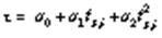 (51) (51)
where t is an estimate of optimal return time, tz,i is initial zone temperature at the beginning of the return period, and a0, a1, and a2 are empirical parameters. The parameters of Equation (51) may be estimated by applying linear least-squares techniques to the difference between the actual return time and the estimates. These parameters may be continuously corrected using recursive updating schemes as outlined by Ljung and Söderström (1983).
For heating, Seem et al. found that ambient temperature has a significant effect on the return time and that the following relationship works well in correlating return times:
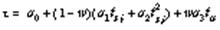 (52) (52)
where ta is the ambient temperature, a0, a1, a2, and a3 are empirical parameters, and w is a weighting function given by
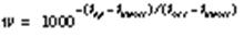 (53) (53)
where tunocc and tocc are the zone set points for unoccupied and occupied periods. Within the context of Equation (52), this function weights the outdoor temperature more heavily when the initial zone temperature is close to the set-point temperature during the unoccupied time. Again, the parameters of Equation (52) may be estimated by applying linear least-squares techniques to the difference between the actual return time and the estimates.
Ideally, separate equations should be used for zones that have significantly different return times. Equipment operation is initiated for the zone with the earliest return time. In a building with a central cooling system, the equipment should be operated above some minimum load limit. With this constraint, some zones need to be returned to their set points earlier than the optimum time.
Optimal start algorithms often use a measure of the building mass temperature rather than the space temperature to determine return time. Although use of space temperature results in lower energy costs (i.e., shorter return time), the mass temperature may result in better comfort conditions at the time of occupancy.
Emergency Strategy to Limit Peak Cooling Requirements
Keeney and Braun (1997) developed a simple control strategy that uses building thermal mass to reduce peak cooling requirements in the event of a loss of a chiller. This emergency strategy is used only on days where cooling capacity is not sufficient to keep the building in the comfort range using night setup control. It involves precooling the building during unoccupied times and allowing the temperature to float through the comfort zone during occupancy.
The precooling control strategy is depicted in Figure 36 along with conventional night setup control. Precooling is controlled at a constant temperature set point, tpre. The warm-up period is used to reset the zone air temperature set point so that the cooling system turns off without calling for heating. During this time, the zone air warms due to lighting and equipment loads. The occupied set point (tocc) is set at the low end of the comfort region so that the building mass charge is held as long as cooling capacity is available. This set point is maintained until the limit on cooling capacity is reached. After this point, the temperatures in the zones float up and the building thermal mass provides additional cooling. If the precooling and occupied set points have been chosen properly and the cooling capacity is sufficient, the zone conditions will remain comfortable throughout the occupied period. The peak cooling requirement can be reduced by as much as 25% using this strategy as compared with night setup control. Thus, the loss of one of four identical chillers could be tolerated. This strategy could also be used for spaces such as auditoriums that have a high occupancy density for a short period.
The length of time and temperature for precooling and the occupied temperature set point chosen for this strategy strongly influence the capacity reduction and could affect occupant comfort. A reasonable strategy is to precool at 68°F beginning at midnight, allow a 30 min warm-up period before occupancy, and then adjust the occupied set point to 70°F. The zone temperature will then rise above this set point when the chillers are operating at capacity.
Case Study. The control strategy was tested in a 1.4 million square foot office building located near Chicago, Illinois. The facility has two identical buildings with very similar internal gains and solar radiation loads, connected by a large, separately cooled entrance area. During tests, the east building used the existing building control strategy while the west building used the precooling strategy.
Four 900 ton vapor compression chillers normally provide chilled water to the air-handling units. Loss of one chiller results in a 25% reduction of the total capacity. This condition was simulated by limiting the vane position of the two chiller units that cool the west building to 75%. The capacity limitation was imposed directly at the chiller control panels. Set points were provided to local zone controllers from a modern energy management and control system. Chiller cooling loads and zone thermal comfort conditions were monitored throughout the tests.
Consistent with simulation predictions, the precooling control strategy successfully limited the peak load to 75% of the cooling capacity for the west building, while the east building operated at 100% of capacity. Figure 37 shows the total chiller coil load for the east and west buildings for a week of testing in the middle of August 1995. The cooling-coil load profile on Monday is the most dramatic example of the load shifting during this test period. The peak cooling load for this facility often occurs on Monday morning. The cooling limit was achieved on Monday during a period in which a heat emergency had been declared in the city. The severe ambient conditions were compounded by a power outage that caused a loss of the west-side chiller units for approximately 20 min. Under these demanding conditions, the precooling strategy maintained occupant comfort while successfully limiting cooling demand of the west side of the building to less than 75% of that for the east side.
The east-side cooling requirement was at or below the 75% chiller capacity target for Tuesday through Friday so the emergency precooling strategy was not necessary. For these off-design days, the emergency strategy was not effective in reducing the on-peak cooling requirements because discharge of the mass was not initiated when capacity was below the target. The thermal mass remained charged so that peak reduction would occur if the target value on the off-design days was reset to a lower value.
Precooling the top floor of the facility had already been implemented into the conventional control strategy used for the east building. This was necessary to maintain comfort conditions with full cooling capacity on hot days. As a result, even greater peak reduction would have been recorded if the precool strategy had been compared with conventional night setup control. The total electrical use was greater for the precooled west building; however, the strategy was designed for an emergency and does not attempt to minimize costs.
This emergency strategy should only be applied on days when the available cooling capacity is not sufficient to maintain comfort conditions when using night setup control. Otherwise, the costs of providing cooling could increase significantly. Ongoing ASHRAE research is seeking to develop simplified strategies for optimal control of building zone set points to minimize operating costs.
Control of Cool Thermal Storage
The choice of a control strategy for a thermal storage system results from a tradeoff between performance (i.e., operating costs) and ease of implementation (i.e., initial costs). Chiller-priority control has the lowest implementation costs, but generally leads to the highest operating costs. Storage-priority strategies provide superior performance, but require the use of a forecaster and a measurement of state of charge for storage. The rest of this section presents details of chiller-priority, load-limiting, and a rule-based control applied to ice storage systems. Each of these strategies shares the same procedures for charging storage, but differs in the manner in which storage is discharged. In general, the control strategies presented in this section are appropriate for systems with utility rate structures that include time-of-use energy and demand charges, but would not be appropriate in conjunction with real-time pricing. Additional information on control strategies for cool storage systems can be found in Chapter 34, Thermal Storage.
Charging Strategies
Ice making should be initiated when both the building is unoccupied and off-peak electrical rates are in effect. During the ice-making period, the chiller should operate at full capacity. Cooling plants for ice storage generally operate most efficiently at full load because of the auxiliaries and the characteristics of ice-making chillers. With feedback control of the chilled-water/glycol supply temperature, full capacity control is accomplished by establishing a low enough set point to ensure this condition (e.g., 20°F).
Internal Melt Storage Tanks. The chiller should operate until the tank reaches its maximum state of charge or the charging period (i.e., off-peak, unoccupied period) ends. This strategy ensures that sufficient ice will be available for the next day without the need for a forecaster. Typically, only a small heat transfer penalty is associated with restoring a partially discharged, internal melt storage tank to a full charge. For this type of storage device, the charging cycle always starts with a high transfer effectiveness because water surrounds the tubes regardless of the amount of ice melted. The heat transfer effectiveness drops gradually until the new ice formations intersect with old formations, at which point the tank is fully recharged.
External Melt Storage Tanks. These tanks have a more significant heat transfer penalty associated with recharging after a partial discharge because ice forms on the outside of existing formations during charging. In this case, it is more efficient to fully discharge the tank each day and only recharge as necessary to meet the next day’s cooling requirements. To ensure that adequate ice is available, the maximum possible storage capacity needed for the next day must be forecast. The storage requirements for the next day depend on the discharge strategy used and the building load. In general, the state of charge for storage necessary to meet the next day’s load can be estimated according to
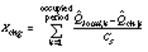 (54) (54)
where Xchg is the relative state of charge at the end of the charging period, Cs is the maximum change in internal energy of the storage tank that can occur during a normal discharge cycle, and Qload,k and Qch,k are forecasts of the building load and chiller cooling requirement for the kth stage (e.g., hour) of the occupied period. The relative state of charge is defined in terms of two reference states: the fully discharged and fully charged conditions that correspond to values of zero and one. These conditions are defined for a given storage based on its particular operating strategy (ASHRAE 1997; Elleson 1996). The fully charged condition exists when the control stops the charge cycle as part of its normal sequence. Similarly, the fully discharged condition is the point where no more usable cooling is recovered from the tank. Typically, zero state of charge corresponds to a tank of water at a uniform temperature of 32°F and a complete charge is associated with a tank having maximum ice build at 32°F. (The fully discharged and fully charged conditions are arbitrarily selected reference states.) In abnormal circumstances, a storage tank can be discharged or charged beyond these conditions, resulting in relative states of charge below zero or above one.
Hourly forecasts of the next day’s cooling requirement can be determined using the algorithm described in the section on Forecasting Diurnal Energy Requirements. However, long-term forecasts are highly uncertain and a safety factor based on previous forecast errors is appropriate (e.g., uncertainty of two or three times the standard deviation of the errors of previous forecasts). Estimates of hourly chiller requirements should be determined using the intended discharge strategy (described in the next section) and building load forecasts.
Discharging Strategies
Three discharge strategies are presented for use with utility structures having on-peak and off-peak energy and demand charges: (1) chiller-priority control, (2) storage-priority, load-limiting control, and (3) a rule-based strategy that uses both chiller-priority and load-limiting strategies.
Chiller-Priority Discharge. During the storage discharge mode, the chiller operates at full cooling capacity (or less if sufficient to meet the load) and storage matches the difference between the building requirement and chiller capacity. For the example system illustrated in Figure 14, the chiller supply temperature set point tchws is set equal to the desired supply temperature for the coils tcoil. If the capacity of the chiller is sufficient to maintain this set point, then storage is not used and the system operates in the direct chiller mode. Otherwise, the storage control valve modulates the flow through storage to maintain the supply set point, providing a cooling rate that matches the difference between the building load and the maximum cooling capacity of the chillers.
This strategy is easy to implement and does not require a load forecast. It works well for design conditions, but can result in relatively high demand and energy costs for off-design conditions because the chiller operates at full capacity during the on-peak period.
Storage-Priority, Load-Limiting Control. Several storage-priority control approaches ensure that storage is not depleted prematurely. Braun (1992) presented a storage-priority control strategy, termed load-limiting control, which tends to minimize the peak cooling plant power demand. The operation of equipment for load-limiting control during different parts of the occupied period can be described as follows:
- Off-Peak, Occupied Period. During this period, the goal is to minimize the use of storage, and the chiller-priority described in the previous section should be applied.
- On-Peak, Occupied Period. During this period, the goal is to operate the chillers at a constant load while discharging the ice storage such that the ice is completely melted when the off-peak period begins. This requires the use of a building cooling-load forecaster. At each decision interval (e.g., 15 min), the following steps are applied:
(1) Forecast the total integrated building cooling requirement until the end of the discharging period.
(2) Estimate the state of charge of the ice-storage tank from measurements.
(3) At any time, the chiller loading for load-limiting control is determined as
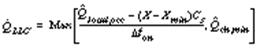 (55) (55)
where Qload,occ is a forecast of the integrated building load for the rest of the on-peak period, Dton is the time remaining in the on-peak period, X is the current state of charge defined as the fraction of the maximum storage capacity, Xmin is a minimum allowable state of charge, Cs is the maximum possible energy that could be added to storage during discharge, and Qch,min is the minimum allowable chiller cooling capacity. If the chiller does not need to be operated during the remainder of the occupied, on-peak period, the minimum allowable cooling capacity could be set to zero. Otherwise, the cooling capacity should be set to the minimum at which the chiller can safely operate.
(4) Determine the chiller set-point temperature necessary to achieve the desired loading as
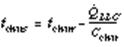 (56) (56)
where tchwr is the temperature of water/glycol returned to the chiller and Cchw is the capacitance rate (mass flow times specific heat) of the flow stream.
Hourly forecasts of cooling loads can be determined using the algorithm described in the section on Forecasting Diurnal Energy Requirements. The hourly forecasts are then integrated to give a forecast of the total cooling requirement. To ensure sufficient cooling capacity, a worst-case forecast of cooling requirements could be estimated as the sum of the best forecast and two or three times the standard deviation of the errors of previous forecasts.
Rule-Based Controller. Drees and Braun (1996) presented a rule-based controller that combines elements of chiller-priority and storage-priority strategies, along with a demand-limiting algorithm to achieve near-optimal control. The demand-limiting algorithm requires a measurement of the total building electrical use. A simpler strategy is described here that does not require this measurement and yields equivalent performance whenever the peak demand for the billing period is coincident with the peak cooling load.
Figure 38 shows a flowchart for the discharge strategy that is applied during each decision interval (e.g., 15 min) during the occupied period. Block 1 determines whether the use of storage should be maximized or minimized. Block 2 is used if the use of storage lowers daily energy costs and storage is sufficient to meet the remainder of the load for the occupied period without operating the chillers. Otherwise, the goal of the strategy in Block 3 is to minimize the use of storage while keeping the peak load below a limit. This strategy tends to keep the chiller(s) heavily loaded (and therefore operating efficiently) until they are no longer needed. The logic in each block is as follows:
- Block 1: Discharge Strategy Selection. The discharge of storage will not reduce the energy cost whenever the cost of replenishing the ice is greater than the cost of providing direct cooling by the chiller(s). This situation is always the case during the off-peak, occupied period because the electricity rates are the same as those associated with the charging period and chillers are less efficient in ice-making mode than when providing direct cooling. Furthermore, during the on-peak, occupied period, using storage generally reduces energy costs whenever the following criterion holds:
ECR > COPd/COPc (57)
where ECR is the ratio of on-peak to off-peak energy charges and COPd and COPc are coefficients of performance for the cooling plant (including chiller, pumps, and cooling tower fans) during discharging and charging of the tank. The COPs should be evaluated at the worst-case charging and discharging conditions associated with the design day. Typically, this ratio is between about 1.2 and 1.8 for systems with cooling towers. However, the ratio can be lower due to the effect of cool nighttime temperatures, especially for systems with air-cooled condensers in dry climates.
If the criterion of Equation (57) is satisfied, control will switch from chiller-priority to storage-priority strategy whenever the storage capacity is greater than the remaining integrated load. Therefore, storage-priority control is enabled whenever
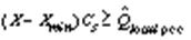 (58) (58)
Hourly forecasts of cooling loads can be determined using the algorithm described in the section on Forecasting Diurnal Energy Requirements and then integrated to give a forecast of the total cooling requirement. To ensure that adequate ice is available, worst-case hourly forecasts can be determined by adding the expected value of the hourly forecasts and the forecast errors associated with a specified confidence interval (e.g., two standard deviations for a 95% confidence interval). The worst-case hourly forecasts can then be integrated to give a worst-case integrated forecast.
- Block 2: Maximum Use of Storage. In this mode, the chillers are turned off and storage is used to meet the entire load throughout the remainder of the occupied period. However, a chiller may need to be turned on if the storage discharge rate is not sufficient to meet the building load (i.e., the coil supply temperature set point can not be maintained).
- Block 3: Minimize Use of Storage with Peak Load Limiting. At any time, a target chiller load is determined as
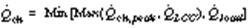 (59) (59)
where Qch,peak is the peak chiller cooling requirement that has occurred during the on-peak period for the current billing period, QLCC is the chiller load associated with load-limiting control and determined with Equation (55), and Qload is the current building load. The chiller set-point temperature necessary to achieve the desired loading is determined as
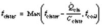 (60) (60)
On the first day of each billing period, Qch,peak is set to zero. For this first day, applying Equation (37) leads to the load-limiting control strategy described in the previous section. On subsequent days, load-limiting control is used only if the current peak limit would lead to premature depletion of storage. Whenever the current load is less than Qch,peak and QLCC, Equations (59) and (60) lead to chiller-priority control.
Forecasting Diurnal Energy Requirements
As discussed previously, forecasts of cooling requirements and electrical use in buildings are often necessary for the control of thermal storage to shift electrical use from on-peak to off-peak periods. In addition, forecasts can help plant operators anticipate major changes in operating modes, such as bringing additional chillers on-line.
In most methods, future predictions are estimated as a function of time-varying input variables that affect cooling requirements and electrical use. Examples of inputs that affect building energy use include: (1) ambient dry-bulb temperature, (2) ambient wet-bulb temperature, (3) solar radiation, (4) building occupancy, and (5) wind speed. Methods that include time-varying measured input variables are often termed deterministic methods.
Not all inputs affecting cooling requirements and electric use are easily measured. For instance, building occupancy is difficult to determine and solar radiation measurements are expensive. In addition, the accuracy of forecast models that use deterministic inputs depends on the accuracy of future predictions of the inputs. As a result, most inputs that affect building energy use are typically not used.
Much of the time-dependent variation in cooling loads and electrical use for a building can be captured with time as a deterministic input. For instance, building occupancy follows a regular schedule that depends on time of day and time of year. In addition, variations in ambient conditions follow a regular daily and seasonal pattern. Many forecasting methods use time in place of unmeasured deterministic inputs in a functional form that captures the average time dependence of the variation in energy use.
A deterministic model has limited accuracy for forecasts due to both unmeasured and unpredictable (random) input variables. Short-term forecasts can be improved significantly by adding previous values of deterministic inputs and previous output measurements (cooling requirements or electrical use) as inputs to the forecasting model. The time history of these inputs provides valuable information about recent trends in the time variation of the forecasted variable and the unmeasured input variables that affect it. Most forecasting methods use variables that reflect past history to predict the future.
Any forecasting method requires that a functional form is defined and the parameters of the model are learned based on measured data. Either offline or online methods can be used to estimate parameters. Offline methods involve estimating parameters from a batch of collected data. Typically, parameters are determined by minimizing the sum of squares of the forecast errors. The parameters of the process are assumed to be constant over time in the off-line methods. Online methods allow the parameters of the forecasting model to vary slowly with time. Again, the sum of squares of the forecast errors is minimized, but sequentially or recursively. Often, a forgetting factor is used to give additional weight to the recent data. The ability to track time-varying systems can be important when forecasting cooling requirements or electric use in buildings because of the influence of seasonal variations in weather.
Forrester and Wepfer (1984) presented a forecasting algorithm that uses current and previous ambient temperatures and previous loads to predict future requirements. Trends on an hourly time scale are accounted for with measured inputs for a few hours preceding the current time. Day-to-day trends are considered by using the value of the load that occurred 24 h earlier as an input. One of the major limitations of this model is its inability to accurately predict loads when an occupied day (e.g., Monday) follows an unoccupied (e.g., Sunday) or when an unoccupied day follows an occupied day (e.g., Saturday). The cooling load for a particular hour of the day on a Monday depends very little on the requirement 24 h earlier on Sunday. Forrester and Wepfer (1984) described a number of methods for eliminating this 24 h indicator. MacArthur et al. (1989) also presented a load profile prediction algorithm that uses a 24 h regressor.
Armstrong et al. (1989) presented a very simple method for forecasting either cooling or electrical requirements that does not use the 24 h regressor; Seem and Braun (1991) further developed and validated this method. The “average” time-of-day and time-of-week trends are modeled using a lookup table with time of day and type of day (e.g., occupied versus unoccupied) as the deterministic input variables. Entries in the table are updated using an exponentially weighted, moving-average model. Short-term trends are modeled using previous hourly measurements of cooling requirements in an autoregressive (AR) model. Model parameters adapt to slow changes in system characteristics. The combination of updating the table and modifying model parameters works well in adapting the forecasting algorithm to changes in season and occupancy schedule.
Kreider and Wang (1991) used artificial neural networks (ANNs) to predict energy consumption of various HVAC equipment in a commercial building. Data inputs to the ANN included (1) previous hour's electrical power consumption, (2) building occupancy, (3) wind speed, (4) ambient relative humidity, (5) ambient dry-bulb temperature, (6) previous hour’s ambient dry-bulb temperature, (7) two hours’ previous ambient temperature, and (8) sine and cosine of the hour number to roughly represent the diurnal change of temperature and solar insolation. The primary purpose in developing these models was to detect changes in equipment and system performance for monitoring purposes. However, the authors suggested that an ANN-based predictor might be valuable when used to predict energy consumption in the future with a network based on recent historical data. Forecasts of all deterministic input variables are necessary to apply this method.
Gibson and Kraft (1993) used an ANN to predict building electrical consumption as part of the operation and control of a thermal energy storage (TES) cooling system. The ANN used the following inputs: (1) electric demand of occupants (lighting and other loads), (2) electric demand of TES cooling tower fans, (3) outside ambient temperature, (4) outside ambient temperature-inside target temperature, (5) outside ambient relative humidity, (6) on-off status for building cooling, (7) cooling system on-off status, (8) Chiller #1 direct-cooling mode on-off status, (9) chiller #2 direct-cooling mode on-off status, (10) ice storage-discharging mode on-off status, (11) ice storage-charging mode on-off status, (12) chiller #1 charging mode on-off status, and (13) chiller #2 charging mode on-off status. To use this forecaster, values of each of these inputs must be predicted. Although the authors suggest that average occupancy demand profile be used as an input, they do not state how the other input variables should be forecast.
A Forecasting Algorithm
This section presents an algorithm for forecasting hourly cooling requirements or electrical use in buildings that is based on the method developed by Seem and Braun (1991). At a given hour n, the forecast value is
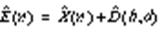 (61) (61)
where
E(n) = forecast cooling load or electrical use for hour n
X(n) = stochastic or probabilistic part of forecast for hour n
D(h,d) = deterministic part of forecast at hour n associated with hth hour of day and current day type d
The deterministic part of the forecast is simply a lookup table for the forecasted variable in terms of hour of the day h and the type of day d. Seem and Braun recommend using three distinct day types: unoccupied days, occupied days following unoccupied days, and occupied days following occupied days. The three day types account for differences between the building responses associated with return from night setup and return from weekend setup. The building operator or control engineer must specify the number of day types and a calendar of day types.
Given the hour of the day and the day type, the deterministic part of the forecast is simply the value stored in that location in the table. Table entries are updated when a new measurement becomes available for that hour and day type. Updates are accomplished through the use of an exponentially weighted, moving-average (EWMA) model as
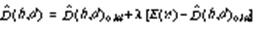 (62) (62)
where
E(n) = measured value of cooling load or electrical use for current hour n
l = exponential smoothing constant, 0 < l < 1
D(h,d)old = previous table entry for D(h,d)
As l increases, the more recent observations have more influence on the average. As l approaches zero, the table entry approaches the average of all data for that hour and day type. When l equals one, the table entry is updated with the most recent measured value. Seem and Braun recommend using a value of 0.30 for l in conjunction with three day types and 0.18 with two day types.
The stochastic portion of the forecast is estimated with a third-order autoregressive model, AR(3), of forecasting errors associated with the deterministic model. With this model, an estimate of the next hour’s error in the deterministic model forecast is given by the following equation:
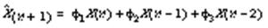 (63) (63)
where
X (n) = difference between measurement and deterministic forecast of cooling load or electrical use at any hour n
f1, f2, f3 = parameters of AR(3) model that must be learned
The error in the deterministic forecast at any hour is simply
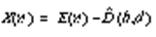 (64) (64)
For forecasting more than one hour ahead, conditional expectation is used to estimate the deterministic model forecast errors using the AR(3) model as follows:
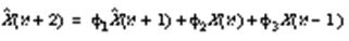
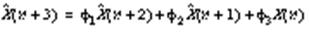

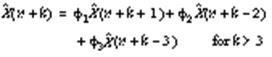 (65) (65)
Online estimation of the AR(3) model parameters is accomplished by minimizing the following time-dependent cost function:
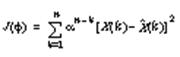 (66) (66)
where the constant a is called the forgetting factor and has a value between 0 and 1. With this formulation, the residual for the current time step has a weight of one and the residual for k time steps back has a weight of a k. By choosing a value of a that is positive and less than one, recent data have greater influence on the parameter estimates. In this manner, the model can track changes due to seasonal or other effects. Seem and Braun recommend using a forgetting factor of 0.99. Parameters of the AR(3) model should be updated at each hour when a new measurement becomes available.
Ljung and Söderström (1983) describe online estimation methods for determining coefficients of an AR model. The parameter estimates should be evaluated for stability. If an AR model is not stable, then the forecasts will grow without bound as the time of forecasts increases. Ljung and Söderström discuss methods for checking stability.
Seem and Braun compared forecasts of electrical usage with both simulated and measured data. Figure 39 shows the standard deviation of the 1 h through 24 h errors in electrical use forecasts for annual simulation results. Results are given for the deterministic model alone, deterministic plus AR(2), and deterministic plus AR(3). For the combined models, the standard deviation of the residuals increases as the forecast length increases. For short time steps (i.e., less than 6 h), the combined deterministic and stochastic models provide much better forecasts than the purely deterministic model (i.e., lookup table).
Seem and Braun also investigated a method for adjusting the deterministic forecast based on using Weather Service forecasts of maximum daily ambient temperature as an input. For short periods (i.e., less than 4 h), forecasts for the temperature-dependent model were nearly identical to forecasts for the temperature-independent model. For longer periods, the temperature-dependent model provided better forecasts than the temperature-independent model.
PREDICTIVE Control Strategies
Model predictive controls applied to commercial buildings require short-term weather forecasts to optimally adjust setpoints in a supervisory control environment. Review of the literature reveals that several researchers are convinced that nonlinear forecasting models based on neural networks (NN) provide superior performance over traditional time series analysis. Florita and Henze (2009) seeks to identify the complexity required for short-term weather forecasting in the context of a model predictive control environment. Moving average (MA) models with various enhancements and neural network models are used to predict weather variables seasonally in numerous geographic locations. Their performance is statistically assessed utilizing the coefficient-of-variation (CV) and the mean bias error (MBE) values. When used in a cyclical two-stage model predictive control process of policy planning followed by execution, the results show that even the most complicated nonlinear autoregressive neural network with exogenous input (NARX) does not appear to warrant the additional efforts in forecasting model development and training in comparison to the simpler MA models.
Field testing of predictive control strategies have carried for both passive and active thermal storage systems (Krarti et al, 2007 and Morgan and Krarti, 2010). In particular, Morgan and Krarti (2010) have investigated the performance of various control strategies for combined passive and active TES systems is through field carried out in an elementary school in Colorado equipped with an ice storage system. The predictive optimal control strategies have been developed using An EnergyPlus-based simulation environment (Zhou et al. 2005, Krarti et al. 2007). The simulation environment was found to be effective in defining and implementing predictive optimal controls for both passive and active TES systems for the buildings. Figures 40 and 41 show examples of the field testing results for the building energy use for performed by Morgan and Krarti (2010).
References
ABMA. 1998. Guideline for the integration of boilers and automated control systems in heating applications. American Boiler Manufacturers Association, Arlington, VA.
Andresen, I. and M.J. Brandemuehl. 1992. Heat storage in building thermal mass: A parametric study. ASHRAE Transactions 98(1).
Armstrong, P.R., T.N. Bechtel, C.E. Hancock, S.E. Jarvis, J.E. Seem, and T.E. Vere. 1989. Environment for structured implementation of general and advanced HVAC controls—Phase II. Small Business Innovative Research Program, Chapter 7. DOE Contract DE-AC02-85ER 80290.
ASHRAE. 2000. Method of testing the performance of cool storage systems. ANSI/ASHRAE Standard 150-2000.
BEI. 1991. Boiler efficiency improvement. Boiler Efficiency Institute, Auburn, AL.
Bellman, R. 1957. Dynamic programming. Princeton University Press, Princeton, NJ.
Bloomfield, D.P. and D.J. Fisk. 1977. The optimization of intermittent heating. Buildings and Environment 12:43-55.
Brandemuehl, M.J., and J. Bradford. 1998. . ASHRAE Research Project 823-RP.
Braun, J.E. 1988. Methodologies for the design and control of central cooling plants. Ph.D. dissertation, University of Wisconsin-Madison.
Braun, J.E. 1990. Reducing energy costs and peak electrical demands through optimal control of building thermal storage. ASHRAE Transactions 96(1).
Braun, J.E. 1992. A comparison of chiller-priority, storage-priority, and optimal control of an ice-storage system. ASHRAE Transactions 98(1): 893-902.
Braun, J.E. and G.T. Diderrich. 1990. Near-optimal control of cooling towers for chilled-water systems. ASHRAE Transactions 96(2):806-813.
Braun, J.E., S.A. Klein, J.W. Mitchell, and W.A. Beckman. 1989a. Applications of optimal control to chilled water systems without storage. ASHRAE Transactions 95(1).
Braun, J.E., S.A. Klein, J.W. Mitchell, and W.A. Beckman. 1989b. Methodologies for optimal control to chilled water systems without storage. ASHRAE Transactions 95(1).
Braun, J.E., J.W. Mitchell, S.A. Klein, and W.A. Beckman. 1987. Performance and control characteristics of a large central cooling system. ASHRAE Transactions 93(1):1830-1852.
Braun, J.E., K.W. Montgomery, and N. Chaturvedi. 2001. Evaluating the performance of building thermal mass control strategies. International Journal of HVAC&R Research 7(4):403-428.
Braun J, 2007a, “A Near-Optimal Control Strategy for Cool Storage Systems with Dynamic Electric Rates”, HVAC&R Journal, 13(4), 557-580.
Braun J., 2007b, “Impact of Control on Operating Costs for Cool Storage Systems with Dynamic Electric Rates”, ASHARE Transactions, Vol. 113.
Braun J, 2007c, “Near-Optimal Control Strategies for Hybrid Cooling Plants”, HVAC&R Journal, 13(4), 599-622.
Braun J, 2007d, “A General Control Algorithm for Cooling Towers in Cooling Plants with Electric and/or Gas-Driven Chillers”, HVAC&R Journal, 13(4), 581-598.
Brent, R.P. 1973. Algorithms for minimization without derivatives, Chapter 5. Prentice Hall.
Brothers, P.W. and M.L. Warren. 1986. Fan energy use in variable air volume systems. ASHRAE Transactions 92(2).
Cheng, H., M.J. Brandemuehl, G.P. Henze, A.R. Florita, and C. Felsmann (2008) “Evaluation of the Primary Factors Impacting the Optimal Control of Passive Thermal Storage (1313-RP).” ASHRAE Transactions, Technical Paper, Vol. 114, Pt. 2, pp. 57-64.
Cumali, Z. 1988. Global optimization of HVAC system operations in real time. ASHRAE Transactions 94(1).
Cumali, Z. 1994. Application of real-time optimization to building systems. ASHRAE Transactions 100(1).
Drees, K.H. 1994. Modeling and control of area-constrained ice storage systems. M.S. thesis, Purdue University, West Lafayette, IN.
Drees, K.H. and J.E. Braun. 1995. Modeling of area-constrained ice storage tanks. International Journal of HVAC&R Research 1(2):143-159.
Drees, K.H. and J.E. Braun. 1996. Development and evaluation of a rule-based control strategy for ice storage systems. International Journal of HVAC&R Research 2(4):312-336.
Dyer, D.F. and G. Maples. 1981. Boiler efficiency improvement. Boiler Efficiency Institute. Auburn, AL.
Elleson, J.S. 1996. Successful cool storage projects: From planning to operation. ASHRAE.
Englander, S.L. and L.K. Norford. 1992. Saving fan energy in VAV systems, Part 2: Supply fan control for static pressure minimization using DDC zone feedback. ASHRAE Transactions 98(1):19-32.
Florita, A.R. and G.P. Henze (2009) “Comparison of Short-Term Weather Forecasting Models for Model Predictive Control.” HVAC&R Research, Vol. 15, Pt. 5, pp. 835-853.
Forrester, J.R. and W.J. Wepfer. 1984. Formulation of a load prediction algorithm for a large commercial building. ASHRAE Transactions 90(2B): 536-551.
Gibson, G.L. and T.T. Kraft. 1993. Electric demand prediction using artificial neural network technology. ASHRAE Journal 35(3):60-68.
Greenfelder, E.M., G.P. Henze, and C. Felsmann (2010) “An Investigation of Optimal Control of Passive Building Thermal Storage with Real Time Pricing.” Manuscript submitted to Journal of Building Performance Simulation.
Grumman, D.L. and A.S. Butkus, Jr. 1988. Ice storage application to an Illinois hospital. ASHRAE Transactions 94(1):1879-1893.
Hackner, R.J., J.W. Mitchell, and W.A. Beckman. 1984. HVAC system dynamics and energy use in buildings—Part I. ASHRAE Transactions 90(2B):523-535.
Hackner, R.J., J.W. Mitchell, and W.A. Beckman. 1985. HVAC system dynamics and energy use in buildings—Part II. ASHRAE Transactions 91(1B):781.
Hartman, T. 1993. Terminal regulated air volume (TRAV) systems. ASHRAE Transactions 99(1):791-800.
Henze, G.P., M. Krarti, and M.J. Brandemuehl. 1997a. A simulation environment for the analysis of ice storage controls. International Journal of HVAC&R Research 3(2):128-148.
Henze, G.P., M. Krarti, and M.J. Brandemuehl. 2003. Guidelines for improved performance of ice storage systems. Energy and Buildings 35(2):111-127.
Henze, G.P., R.H. Dodier, and M. Krarti. 1997b. Development of a predictive optimal controller for thermal energy storage systems. International Journal of HVAC&R Research 3(3):233-264.
Henze, G.P., D. Kalz, S. Liu, and C. Felsmann (2005) “Experimental Analysis of Model-Based Predictive Optimal Control for Active and Passive Building Thermal Storage Inventory." HVAC&R Research, Vol. 11, No. 2, pp. 189-214.
Henze, G.P., M.J. Brandemuehl, C. Felsmann, A. Florita, and H. Cheng (2007) “Final Project Report for ASHRAE Research Project 1313-RP: Evaluation of Building Thermal Mass Savings.” American Society of Heating, Refrigerating, and Air-Conditioning Engineers, Atlanta, Georgia.
Henze, G.P., C. Felsmann, A.R. Florita, M.J. Brandemuehl, H. Cheng, and C.E. Waters (2008) “Optimization of Building Thermal Mass Control in the Presence of Energy and Demand Charges (1313-RP).” ASHRAE Transactions, Technical Paper, Vol. 114, Pt. 2, pp. 75-84.
Henze, G.P., A.R. Florita, M.J. Brandemuehl, C. Felsmann and H. Cheng (2009) “Advances in Near-Optimal Control of Passive Building Thermal Storage.” Proceedings of the ASME 3rd International Conference on Energy Sustainability, July 19-23 2009, San Francisco, CA.
Kao, J.Y. 1985. Control strategies and building energy consumption. ASHRAE Transactions 91(2).
Keeney, K.R. and J.E. Braun. 1996. A simplified method for determining optimal cooling control strategies for thermal storage in building mass. International Journal of HVAC&R Research 2(1):1-20.
Keeney, K.R. and J.E. Braun. 1997. Application of building precooling to reduce peak cooling requirements. ASHRAE Transactions 103(1):463-469.
Krarti, M., M.J. Brandemuehl, and G.P. Henze. 1996. Evaluation of optimal control for ice systems. ASHRAE Research Project 809-RP.
Krarti, M., Henze G. Zhou G., Ihm P., Liu S., and Morgan S., 2007, “Real-Time Predictive Optimal Control of Active and Passive Thermal Energy Storage systems, Final Report”, report to Department of Energy, Contract DE-FC-36-03G)13026.
Kreider, J.F. and X.A. Wang. 1991. Artificial neural networks demonstration for automated generation of energy use predictors for commercial buildings. ASHRAE Transactions 97(2):775-779.
Lau, A.S., W.A. Beckman, and J.W. Mitchell. 1985. Development of computer control—Routines for a large chilled water plant. ASHRAE Transactions 91(1).
Liu, S. and G.P. Henze (2006a) “Experimental Analysis of Simulated Reinforcement Learning Control for Active and Passive Building Thermal Storage Inventory –Part 1: Theoretical Foundation.” Energy and Buildings, Vol. 38, No. 2, February 2006, pp. 142-147.
Liu, S. and G.P. Henze (2006b) “Experimental Analysis of Simulated Reinforcement Learning Control for Active and Passive Building Thermal Storage Inventory – Part 2: Results and Analysis.” Energy and Buildings, Vol. 38, No. 2, February 2006, pp. 148-161.
Ljung, L. and T. Söderström. 1983. Theory and practice of recursive identification. MIT Press, Cambridge, MA.
MacArthur, J.W., A. Mathur, and J. Zhao. 1989. On-line recursive estimation for load profile prediction. ASHRAE Transactions 95(1):621-628.
Morgan, S. and M. Krarti. 2006. Impact of Electricity Rate Structures on Energy Cost Savings of Pre-cooling Controls for Office Buildings. Energy and Buildings, Volume 38.
Morgan S. and M. Krarti, 2010, “Field Testing of Optimal Controls of Passive and Active Thermal Storage”, ASHRAE Transactions 116(1).
Morris, F.B., J.E. Braun, and S. Treado. 1994. Experimental and simulated performance of optimal control of building thermal storage. ASHRAE Transactions 100(1):402-414.
Parker, S.A., R.B. Scollon, and R.D. Smith. 1997. Boilers and fired systems. Energy Management Handbook. Fairmont Press, Lilburn, GA.
Rabl, A. and L.K. Norford. 1991. Peak load reduction by preconditioning buildings at night. International Journal of Energy Research 15:781-798.
Ruud, M.D., J.W. Mitchell, and S.A. Klein. 1990. Use of building thermal mass to offset cooling loads. ASHRAE Transactions 96(2).
Rawlings, L.K. 1985. Strategies to optimize ice storage. ASHRAE Journal 27(5):39-44.
Seem, J.E., P.R. Armstrong, and C.E. Hancock. 1989. Comparison of seven methods for forecasting the time to return from night setback. ASHRAE Transactions 95(2).
Seem, J.E. and J.E. Braun. 1991. Adaptive methods for real-time forecasting of building electrical demand. ASHRAE Transactions 97(1):710-721.
Seem, J.S., C. Park, and J.M. House. 1999. A new sequencing control strategy for air-handling units. International Journal of HVAC&R Research 5(1):35-58.
Snyder, M.E. and T.A. Newell. 1990. Cooling cost minimization using building mass for thermal storage. ASHRAE Transactions 96(2): 830-838.
Spethmann, D.H. 1989. Optimal control for cool storage. ASHRAE Transactions 95(1).
Tamblyn, R.T. 1985. Control concepts for thermal storage. ASHRAE Transactions 91(1B).
Taplin, H.R. 1998. Boiler plant and distribution system optimization manual. Fairmont Press, Lilburn, GA.
Warren, M. and L.K. Norford. 1993. Integrating VAV zone requirements with supply fan operation. ASHRAE Journal 35(4):43-46.
Watkins, C. and P. Dayan (1992) “Q-learning.” Machine Learning Vol. 8, pp. 279–292.
Wei, G., M. Liu, and D.E. Claridge. 2004. Integrated damper and pressure reset for VAV supply air fan control. ASHRAE Transactions 110(2).
Winkelman, F.C., W.F. Buhl, B. Birdsall, A.E. Erdem, K.L. Ellington, and Hirsch & Associates. 1993. DOE-2 BDL summary, version 21.E, LBNL Report 34946, Lawrence Berkeley National Laboratory, Berkeley, CA.
Zhou, G., Ihm, P., Krarti, M., Liu, S., and G.P. Henze, 2005, “Integration of an Internal Optimization Module within EnergyPlus.” IBPSA Proceedings. |
 (1)
(1) (2)
(2) (3)
(3)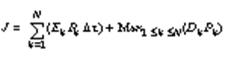 (12)
(12)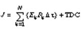 (17)
(17)