Chapter 16 Variance Analysis

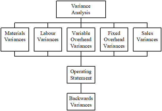
1.       Objectives

1.1       Calculate, identify the cause of and interpret basic variances:
(a)        Sales price and volume, including sales mix and quantity variances.
(b)       Materials total, price and usage, including material mix and yield variances
(c)        Labour total, rate and efficiency
(d)       Variable overhead total, expenditure and efficiency
(e)        Fixed overhead total, expenditure and, where appropriate, volume, capacity and efficiency
1.2       Calculate the effect of idle time and waste on variances including where idle time has been budgeted for.
1.3       Produce full operating statements in both a marginal cost and full absorption costing environment, reconciling actual profit to budgeted profit.
1.4       Identify the causes of labour, material, overhead and sales margin variances.

2.      Standard Costing System

2.1       Standard costing is a technique which establishes predetermined estimated of the costs of products and services and then compares these predetermined costs with actual costs as they are incurred. The predetermined costs are known as standard costs and the difference between the standard cost and actual cost is known as a variance.
2.2       The process by which the total difference between actual cost and standard cost is broken down into its different elements is known as variance analysis.
2.3       It can be used in a variety of costing situations, batch and mass production, process manufacture, transport, certain aspects of repetitive clerical work and even in jobbing manufacture. Undoubtedly, the greatest benefit is gained when the manufacturing method involves a substantial degree of repetition. Its major application in practice is in organizations involved in mass production and/or repetitive assembly work.

2.4       Standard-setting

2.4.1    Standards are set for each element of cost in the production of a unit of output. It provides estimating the quantity of the resource used and its associated costs. In addition a standard selling price is set.
2.4.2    Direct materials
(i)      Product specifications are derived from study (or average past performance).
(ii)     Quantity standards are recorded, for example, as a bill of materials.
(iii)    Standard prices are obtained from the purchasing department which researches alternative suppliers and selects those which can provide:

• Required quantity
• Sound quality
• Most competitive price

2.4.3    Direct labour
(i)      “Time and motion” studies of operations may be used to determine the most efficient production method.
(ii)     Time managements determine standard hours for the average worker to complete a job.
(iii)    Wages rates are determined by company policy/negotiations between management and unions.
2.4.4    Variable overheads
(i)      A standard variable overhead rate per unit of activity is calculated.
(ii)     If there is no observable direct relationship between resources and output, past data is used to predict.
(iii)    The activity measure that exerts the greatest influence on costs is investigated – usually direct labour hours (or machine hours).
2.4.5    Fixed overheads
(i)      Because fixed costs are largely independent of changes in activity, they are constant over wide ranges in the short term.
(ii)     Therefore, for control purposes, a fixed overhead rate per unit of activity is inappropriate.

2.5       Advantages and limitation of standards

2.5.1    Advantages of standards
(i)      Managerial planning – It greats deal in ensuring that all available resources are utilized optimally and so leading to maximize the profits of the enterprise.
(ii)     Coordination – It helps the coordination of different functions such as manufacturing, marketing, engineering, accounting, etc., towards a common goal.
(iii)    Cost control – It helps the company to identify the activities which fail to come up to the standards fixed and those which exceed such standards, through the ‘principle of exception’.
(iv)    Economy in record keeping – Standard costs reduce clerical effort and expense.
(v)     Incentives to employees – Standards motivate the staff to work more efficiently in the accomplishment of company objectives. Many incentives and rewards like cash bonus can be based on actuals as related to standards.
2.5.2    Limitations of standards
(i)      High start-up expenses – Fixing of standards and their implementation calls for substantial expenditure initially.
(ii)     Difficulties in determining standard costs – It involves a high degree of accuracy to determine the standard costs. Thus, a good number of assumptions will have to be made to cover many situations.
(iii)    Implementation in case of some industries poses difficulties – especially in non-standardised products.
(iv)    Opposition from employees – The employees consider the standard costing as an oppressive measure solely intended to extract the maximum from them.

2.6       Overview of principles

2.7       Purposes of standard costing

2.7.1    Standard costing systems are widely used because they provide cost data for many different purposes. The following are the major purposes for which a standard costing system can be used:
(i)      To assist in setting budgets and evaluate managerial performance.
(ii)     To act as control device by highlighting those activities that do not conform to plan, and thus alerting decision-makers to those situations that may be ‘out of control’ and in need of corrective action.
(iii)    To provide a prediction of future costs that can be used for decision-making purposes.
(iv)    To simplify the task of tracing costs to products for inventory valuation purposes.
(v)     To provide a challenging target that individuals are motivated to achieve.

 

 

3.      Variance Analysis

3.1       It will be recalled from the previous section that a variance is the difference between standard cost and actual cost. The process by which the total difference between standard and actual costs is sub-divided is known as variance analysis which can be defined as: “The analysis of variances arising in a standard costing system into their constituent parts.”
3.2       Variances may be ADVERSE (or UNFAVOURABLE), i.e. where actual cost is greater than standard, or they may be FAVOURABLE, i.e. where actual cost is less than standard.
3.3       The only purpose of variance analysis is to provide practical pointers to the causes of off-standard performance so that management can improve operations, increase efficiency, utilize resources more effectively and reduce costs.
3.4       The types of variances which are identified must be those which fulfill the needs of the organization. The only criterion for the calculation of a variance is its usefulness – if it is not useful for management purposes, it should not be produced.

 

3.5       Material variances

3.5.1    A particular problem arises with materials variances in that materials can be charged to production at either actual prices or standard prices. This affects when the price variance is calculated, i.e. either at the time of purchase or at the time of usage.
3.5.2    The procedure where materials are charged to production at standard price has many advantages. This method means that variances are calculated as soon as they arise, and that they are more easily related to an individual’s responsibility (i.e. a price variance would be the buyer’s responsibility).
3.5.3    Formulae for materials variances

1. Total material cost variance	= (SP x SQ – AP x AQ)
2. Material price variance	= (SP – AP) x AQ
3. Material usage variance	= (SQ – AQ) x SP

Where:
SP = Standard Price
AP = Actual Price
SQ = Standard Quantity for actual output
AQ = Actual quantity

 

3.5.5

Materials mix and yield variances

(a)       A mix variance occurs when the materials are not mixed or blended in standard proportions and it is a measure of whether the actual mix is cheaper or more expensive than the standard mix. (Actual quantity at actual mix – actual quantity at standard mix) × standard price (b)       A yield variance arises because there is a difference between what the input should have been for the output achieved and the actual input. (Actual yield – standard yield from actual input of material) × standard cost per unit of output

3.5.6

Example 2

Calculate the material mix variance from the following particulars: Standard mix for product Actual mixture of product A 100 kg @ $60/kg A 90 kg @ $60/kg B 150 kg @ $50/kg B 130 kg @ $50/kg   250 kg     220 kg   Standard quantity for actual production for A = 100/250 x 220 = 88 Standard quantity for actual production for B = 150/250 x 220 = 132 A (88 – 90) x $60 = $120 (Adverse) B (132 – 130) x $50 = $100 (Favourable) Material mix variance = $20 (Adverse)

 

Typical causes of material variances
(a)     Material price variance
(i)      Recent changes in purchase price of materials.
(ii)     Failure to purchase anticipated quantities when standards were established resulting in higher prices owing to non-availability of quantity purchase discounts.
(iii)    Not taking cash discounts anticipated at the time of setting standards resulting in higher prices.
(iv)    Substituting raw material differing from original materials specifications.
(v)     Freight cost changes and changes in purchasing and store-keeping costs if these are debited to the material cost.
(b)     Materials usage variance
(i)      Pool materials handling.
(ii)     Inferior workmanship by machine operator.
(iii)    Faulty equipment.
(iv)    Cheaper, defective raw material causing excessive scrap.
(v)     Inferior quality control inspection.
(vi)    Pilferage.
(vi)    Wastage due to inefficient production method.

3.6       Labour variances

3.6.1    The cost of labour is determined by the price paid for labour and the quantity of labour used. Thus a price and quantity variance will also arise for labour. Unlike materials, labour cannot be stored, because the purchase and usage of labour normally takes place at the same time. Hence the actual quantity of hours purchased will be equal to the actual quantity of hours used for each period. For this reason the price variance plus the quantity variance should agree with the total labour variance.
3.6.2    Idle time may be caused by machine breakdowns or not having work to give to employees, perhaps because of bottlenecks in production or a shortage of orders from customers. When it occurs, the labour force is still paid wages for time at work, but no actual work is done. Such time is unproductive and therefore inefficient.
3.6.3    Formulae for labour variances

1. Labour cost variance	= SR x SH – AR x AH
2. Labour rate variance	= (SR – AR) x AH
3. Labour efficiency variance	= (SH – AH) x SR

Where:
SR = Standard Rate
AR = Actual Rate
SH = Standard Hours
AH = Actual Hours

3.6.4

Example 3

During December, 1,500 units of X were made and the cost of grade Z labour was $17,500 for 3,080 hours. A unit of product X is expected to use 2 hours of grade Z labour at a standard cost of $5 per labour hour. During the period, however, there was a shortage of customer orders and 100 hours were recorded as idle time. Required: Calculate the following variances. (a)        The total labour cost variance (b)       The labour rate variance (c)        The idle time variance (d)       The labour efficiency variance Solution: (a)        The total labour cost variance = 1,500 units × $5 × 2 hours – $17,500 = $2,500 (A) (b)       The labour rate variance = 3,080 hours × $5 – $17,500 = $2,100 (A) (c)        The idle time variance = 100 hours × $5 = $500 (A) (d)       The labour efficiency variance = [1,500 units × 2 hours – (3,080 hours – 100 hours)] × $5 = $100 (F) Summary   $   Labour rate variance 2,100 (A) Idle time variance 500 (A) Labour efficiency variance 100 (F) Total labour cost variance 2,500 (A) Remember that, if idle time is recorded, the actual hours used in the efficiency variance calculation are the hours worked and not the hours paid for.

3.6.5    Typical causes of labour variances
(a)     Labour rate variance
(i)      Employing workers of different wage rates.
(ii)     Changes in the basic wage rates.
(iii)    Use of a different method of wages payment.
(iv)    New workers not being allowed full normal wage rates.
(v)     Unscheduled overtime.
(b)     Labour efficiency variance
(i)      Operator’s ability and efficiency below standard.
(ii)     Incompetent supervision and incorrect instructions.
(iii)    Poor working conditions.
(iv)    Change in the method of operation.
(v)     Machine breakdowns.
(vi)    Increase in labour turnover.

3.7       Variable overhead variances

3.7.1    Overhead cost variance is the difference between the actual overheads incurred and the standard overheads. The overhead cost variance may be defined as ‘the difference the standard cost of overhead absorbed for the output achieved and the actual overhead cost.’
3.7.2    Formulae for variable overhead cost variances

1. Variable overhead variance	= SVO – AVO
2. Variable overhead efficiency variance	= (SH – AH) x SVOR
3. Variable overhead expenditure variance	= (SVOR – AVOR) x AH

Where:
SVO = Standard Variable Overhead
AVO = Actual Variable Overhead
SH = Standard Hours of Output
AH = Actual Hours worked
SVOR = Standard Variable Overhead Rate
AVOR = Actual Variable Overhead Rate

3.8       Fixed overhead cost variances

3.8.1   With a variable costing system, fixed manufacturing overheads are not unitized and allocated to products. Instead, the total fixed overheads for the period are charged as an expense to the period in which they are incurred. Fixed overheads are assumed to remain unchanged in response to changes in the level of activity, but they may change in response to other factors.
3.8.2    Formulae for the calculation of fixed overhead cost variances:

1. Fixed overhead variance	= AbFO – AFO
2. Fixed overhead expenditure variance	= BFO – AFO
3. Fixed overhead volume variance	= AbFO – BFO
4. Volume efficiency variance	= AbFO – SFO
5. Volume capacity variance	= SFO – BFO

Where:
AbFO = Absorbed Fixed Overheads
AFO = Actual Fixed Overheads
BFO = Budgeted Fixed Overheads
SFO = Standard Fixed Overheads

3.8.3

Example 4

The following information was obtained from the records of a manufacturing unit using Standard Costing System:   Budgeted Actual Production per month 2,500 units 2,000 units Assume 8 hours/day     Working days 25 26 Fixed overhead $50,000 $45,000 Variable overhead $15,000 $15,000 Required: To calculate the following overhead variance. (a)        Variable overhead variance (b)       Fixed overhead variance Solution: Working hours available/day = 25 x 8 = 200 hours Standard time =  = 0.08 hr/unit Variable overhead absorption rate = Budgeted variable overhead Planned production in standard hours = $15,000 / 200 hours = $75/hour Fixed overhead absorption rate = Budgeted fixed overhead Planned production in standard hours = $50,000 / 200 hours = $250/hour (a) (i) Variable overhead cost variance   =   SVO – AVO   = 75 x 0.08 x 2,000 – 15,000   = 12,000 – 15,000   = $3,000 (A) (a) (ii) Variable overhead expenditure variance   =   (SVOR – AVOR) x AH   = 75 x 26 x 8 – 5,000   = 15,600 – 15,000   = $600 (F) (a) (iii) Variable overhead efficiency variance   =   (SH – AH) x SVOR   = (2,000 x 0.08 – 208) x 75   = $3,600 (A) (b) (i) Fixed overhead cost variance = AbFO – AFO   = (250 x 0.08 x 2,000) – 45,000   = 40,000 – 45,000   = $5,000 (A) (b) (ii) Fixed overhead expenditure variance   =   BFO – AFO   = 50,000 – 45,000   = $5,000 (F) (b) (iii) Fixed overhead volume variance   =   AbFO – BFO   = 250 x (0.08 x 2,000) – 50,000   = 40,000 – 50,000   = $10,000 (A) (b) (iv) Fixed overhead efficiency variance = = AbFO – SFO FOAR x Actual labour hours worked – FOAR x standard hours for actual output   = 250 x 26 x 8 – 250 x 0.08 x 2,000   = 12,000 (A) (b) (iv) Fixed overhead capacity variance = = AbFO – BFO FOAR x Actual labour hours worked – Budgeted fixed overhead   = 250 x 26 x 8 – 50,000   = 52,000 – 50,000   = 2,000 (F)

 

3.5.4

Example 1

Standard price $15.00 per Kg Actual price $12.00 per Kg Standard quantity 2,000 Kg Actual quantity 1,200 Kg Required: Calculate: (a) Material cost variance, (b) Material price variance, and (c) Material usage variance. Solution: Material cost variance = (SP x SQ – AP x AQ)   = (15 x 2,000 – 12 x 1,200   = 15,600 (F)       Material price variance = (SP – AP) x AQ   = (15 – 12) x 1,200   = 3,600 (F)       Material usage variance = (SQ – AQ) x SP   = (2,000 – 1,200) x 15   = 12,000 (F)       Material cost variance = Material price variance + material usage variance   = 3,600 (F) + 12,000 (F)   = 15,600 (F)

 

Typical causes of overhead volume variance:
(i)         Failure to utilize normal capacity.
(ii)        Lack of sales order.
(iii)       Too much idle capacity.
(iv)       Inefficient or efficient utilization or existing capacity.
(v)        Machine breakdown.
(vi)       Defective materials.
(vii)      Labour troubles.
(viii)     Power failures.

3.9       Sales variances

3.9.1    Sales variances can be used to analyze the performance of the sales function on broadly similar terms to those for manufacturing costs. The most significant feature of sales variance calculations is that they are calculated in terms of profit or contribution margins rather than sales value.
3.9.2    It is important to understand the definition of standard sales margin before we approach sales margin variances. This is defined as the difference between the standard selling price of product of the product and the standard cost of the product. It is also referred to as the standard margin of the product.
3.9.3    Formulae for the calculation of sales variances

1. Total sales margin variance	= AM – BM
2. Sales margin price variance	= (Am – Sm) x AV
3. Sales margin quantity variance	= (AQ – BQ) x SM
4. Sales margin mix variance	= (AQAm – AQSm) x SM
5. Sales margin volume variance	= (AQSm – BSSm) x SM

Where:
AM = Actual Margin
BM = Budgeted Margin
Am = Actual Margin per unit
Sm = Standard Margin per unit
AV = Actual Sales Volume
AQ = Actual Quantity
BQ = Budgeted Quantity
AQAM = Actual Quantity in Actual Mix
AQSM = Actual Quantity in Standard Mix
AQSM = Actual Quantity in Standard Mix
BSSM = Budgeted Sales in Standard Mix

The Operating Statement

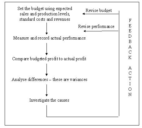
4.1       Top management will be interested in the reason for the actual profit being different from the budgeted profit. By adding the favourable production and sales variances to the budgeted profit and deducting the adverse variances, the reconciliation of budgeted and actual profit is shown as follow.
4.2       The following reconciliation of budgeted and actual profits (using a standard variable costing system) assumes that the company produces a single product consisting of a single operation and that the activities are performed by one responsibility centre. In practice, most companies make many products, which require operations to be carried out in different responsibility centers. A reconciliation statement such as that presented as follow will therefore normally represent a summary of the variances for many responsibility centers. The reconciliation statement thus represents a broad picture to top management that explains the major reasons for any difference between the budgeted and actual profits.

	$	$	$
Budgeted net profit			X
Sales variances:
Sales margin price	X (F/A)
Sales margin quantity	X (F/A)	X (F/A)
Direct cost variances:
Material: Price	X (F/A)
Usage	X (F/A)	X (F/A)
Labour:   Rate	X (F/A)
Efficiency	X (F/A)	X (F/A)
Manufacturing OH variances:
Fixed OH expenditure	X (F/A)
Variable OH expenditure	X (F/A)
Variable OH efficiency	X (F/A)	X (F/A)	X (F/A)
Actual profit			X

5.      “Backwards” Variances

5.1       Examination questions can be set in which the variances are already given and the requirements are to find actual, budget or other data. This implies that students need to have thorough detailed knowledge of how to calculate variances. Essentially the process involved is working backwards with the formula to find missing figures. There is no set approach since questions will not be identical, but the following can act as a guide.
5.2       To find actual production

	$
Actual cost	X
± Variances	X
= Standard cost of actual production	X
¸ Standard cost per unit	X
= Actual production	X

 

 

5.3       To find budget production
Using fixed overhead expenditure variance

	$
Actual fixed overhead	X
Budget fixed overhead	X
Fixed overhead expenditure variance	X

Budget production =	Budgeted fixed overhead
	Standard fixed overhead rate

 

5.4       To find actual data – Use the relevant variance formula containing the actual data required. For example, to find actual price paid per unit of material Þ use material price variance.

5.5

Example 6

Standard cost card     $ Materials 2 kgs at $2 per kg 4 Labour 3 hours at $5 per hour 15 Variable overhead 3 hours at $1 per hour 3 Fixed overhead   1 Standard cost of sales   23 Profit per unit   7 Sales price   30 Additional information     $ Budgeted profit   70,000 Sales volume variance (A)   700 Sales price variance (F)   49,500 Cost variances     Fav Adv     $ $ Materials Price   25,050   Usage   60,400         Labour Rate   6,640   Idle time   1,000   Efficiency (other)   15,750         Variable Total 7,850           Fixed overhead Expenditure   5,000 Actual labour paid = 33,200 hours × $5.20 Actual material purchased = 50,000 kgs Actual fixed overhead = $15,000 Required: Calculate the following: (a)        Actual units produced (b)       Actual price/kg of material (c)        Budget units produced (d)       Actual units sold (e)        Actual profit Solution: (a)        Actual units produced   $ Actual cost of labour (33,200 x 5.2)            172,640 Labour rate             (6,640) Idle time             (1,000) Efficiency           (15,750) Standard cost of actual production            149,250 Standard labour cost/unit                     15 Actual production (units)                9,950     (b)       Actual material price per kg   $ Actual price (bal. fig.)                2.501 Standard price                  2.00                  0.501 x actual purchases              50,000 Material price variance          25,050 A (c)        Budget production = = (15,000 – 5,000) ÷ $1 = 10,000 (d)       Actual units sold   $ Actual sales level (bal. fig.)                9,900 Budget sales level              10,000                     100 x Standard profit/unit                       7 Sales volume variance               700 A (e)        Actual profit   $ Budget profit              70,000 Sales volume variance                (700) Selling price variance              49,500 Cost variances   Material   Price           (25,050) Usage           (60,400) Labour   Rate             (6,640) Efficiency           (16,750) Variable overhead                7,850 Fixed overhead   Expenditure             (5,000) Volume (W)                  (50) Actual profit              12,760 Working   Units Actual volume produced                9,950 Budget volume produced              10,000                       50 x Standard fixed overhead rate                     $1 Fixed overhead volume variance               $50 A

 

3.9.4

Example 5

The budgeted sales and actual sales of XYZ Baby Cot Dealers for its three products for the month of June 2012 are given as below: Product Total sales ($) in ‘000s Budgeted unit Budgeted Margin $ in 000’s Total sales $ in 000’s Actual unit Actual total margin $ in 000’s     Vol Price Margin     Vol Price Margin   P 250 500 500 100 50 275 550 500 100 55 Q 225 300 750 150 45 200 250 800 200 50 R 200 200 1,000 200 40 95 100 950 150 15     1,000     135   900     120 Required: Compute all the sales margin variances. Solution: (i)         Total sales margin variance = Actual margin – Budgeted margin P 550 x 100 – 500 x 100 = 5,000 (F) Q 250 x 200 – 300 x 150 = 5,000 (F) R 100 x 150 – 200 x 200 = 25,000 (A)       15,000 (A) (ii)        Sales margin price variance = (Actual margin – Standard margin) x number of units sold in the period P (100 – 100) x 550 = 0   Q (200 – 150) x 250 = 12,500 (F) R (150 – 200) x 100 = 5,000 (A)       7,500 (F) (iii)       Sales margin quantity variance = (Actual quantity – Budgeted quantity) x Standard margin per unit P (550 – 500) x 100 = 5,000 (F) Q (250 – 300) x 150 = 7,500 (A) R (100 – 200) x 200 = 20,000 (A)       22,500 (A) (iv)       Sales margin mix variance = (Actual quantity in actual mix – Actual quantity in standard mix) x standard margin per unit P (550 – 450) x 100 = 10,000 (F) Q (250 – 270) x 150 = 3,000 (A) R (100 – 180) x 200 = 16,000 (A)       9,000 (A) Actual number of units sold 900 at standard proportions, i.e. 50%, 30% and 20% is 450, 270 and 180. (v)        Sales margin volume variance = (Actual quantity in standard mix – Budgeted sales in standard mix) x standard margin per unit P (450 – 500) x 100 = 5,000 (A) Q (270 – 300) x 150 = 4,500 (A) R (180 – 200) x 200 = 4,000 (A)       13,500 (A)