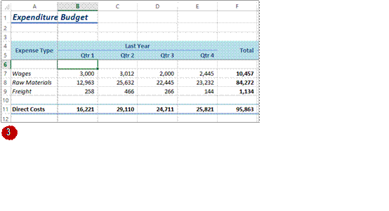
 When you lay out your data in rows and columns, it is most likely that your headings end up at the top or to the left of your data. If you have a large amount of data, you may find that when you
scroll across or down to particular cells, the headings scroll out of view. This problem can be resolved by freezing the rows and/or columns that hold the headings.
Try This Yourself: |
|
Same File |
Continue using the previous file with this exercise, or open the file E1324 Worksheet Techniques_11.xlsx... |
|
Click on the Maintenance worksheet tab, then spend a few moments examining the worksheet |
|
Click in cell B6 to select the cell |
|
Click on the VIEW tab, click on Freeze Panes in the Window group, then select Freeze Panes |
|
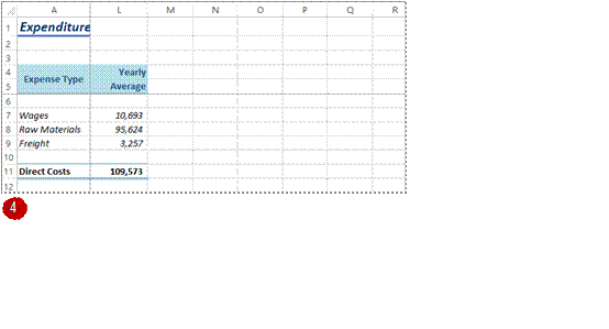
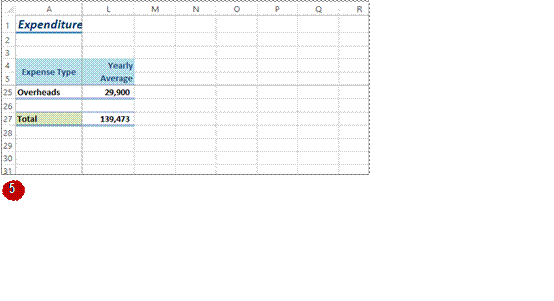
Scroll to the right until Yearly Average in column L appears next to column A |
|
Scroll down until Overheads in row |
|
Press |
|
On the VIEW tab, click on Freeze Panes in the Freeze Panes group, then click on Unfreeze Panes to unfreeze the rows and columns |

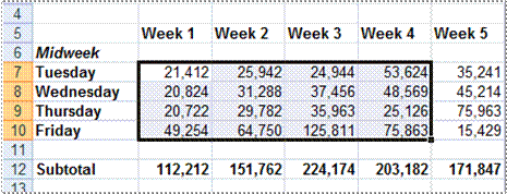
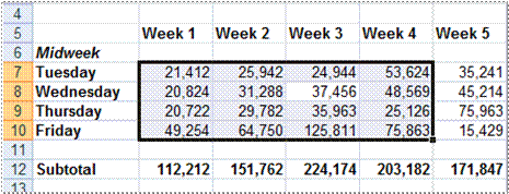
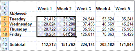
A contiguous range is any group of selected cells that form either a square or a rectangle. A single cell that is selected is also considered to be a range. Ranges can be selected using the
mouse, the keyboard or a combination of the two. Once selected, you can use the range for input, or apply formatting, or copy the cells as required.
![]()
![]()
![]()

ù![]()
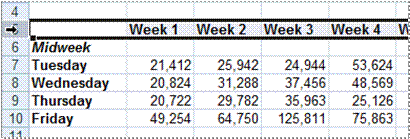
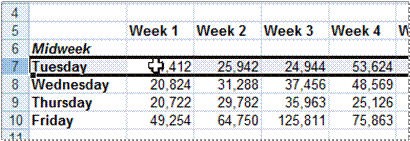
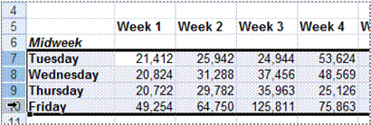
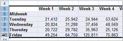
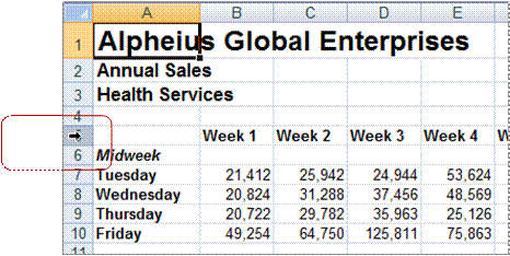 If you want to make changes to an entire row, such as bolding all of the headings in a row or changing the font of all the cell entries, you must first select the row. This is done by clicking on the
row header to the left of the row. Remember that any changes you make will apply to every cell in the row all the way across to column XFD, so be careful!
![]()
![]()
![]()
![]()
Try This Yourself: |
|
Same File |
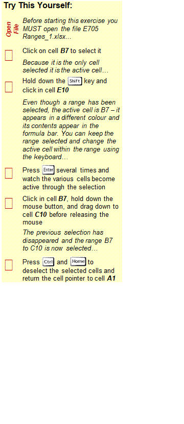
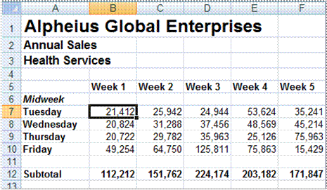
Continue using the previous file with this exercise, or open the file E705 Ranges_1.xlsx... |
|
Press |
|
Move the mouse pointer to the row heading for row 5 |
|
Click once on row heading 5 to select the entire row |
|
Click in cell B7and press |
|
Click on the row header for row 7 |
|
Hold down |
|
Click in the row header for row 5, then hold down the left mouse button and drag down the row headers to row 10 |

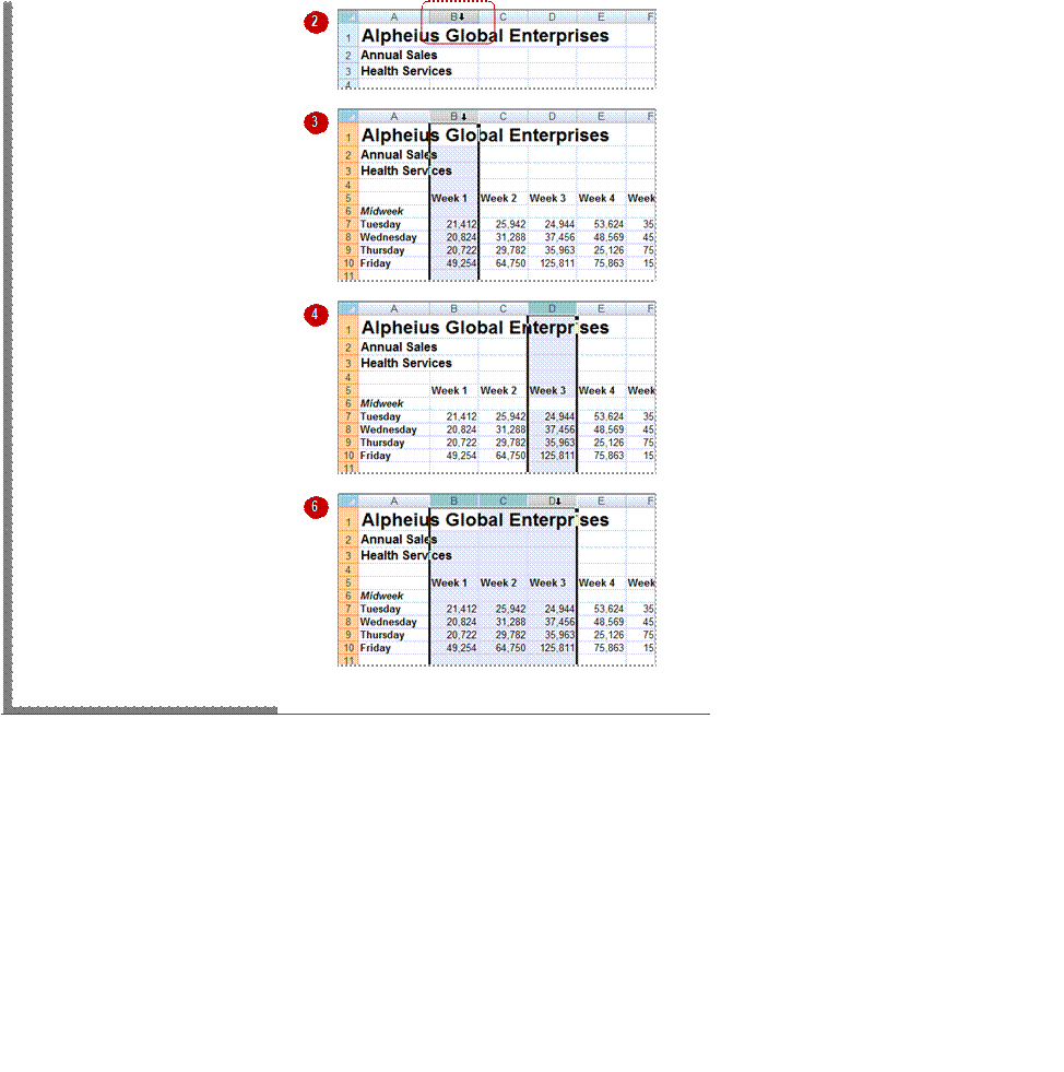
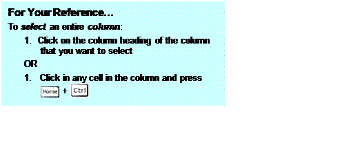
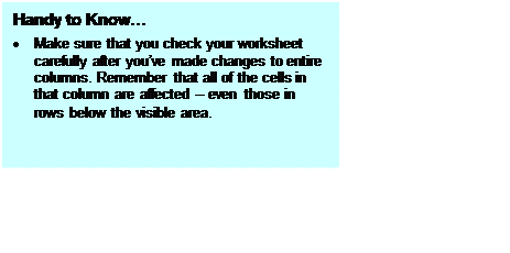
If you want to make changes to an entire column, such as bolding all of the headings in a column or changing the font of all the cell entries, you must first select the column. This is done by
clicking on the column header directly above the column. Remember that any changes you make will apply to every cell in the column all the way down to row 1,048,576!
![]()
![]()
Try This Yourself: |
|
Same File |
Continue using the previous file with this exercise, or open the file E705 Ranges_1.xlsx... |
|
Press |
|
Move the mouse pointer to the column heading for column B |
|
Click once to select the column |
|
Click in cell D6 and press |
|
Click on the column header for column B to select it |
|
Hold down |
|
Click in the column header for column A, then hold down the left mouse button and drag the mouse pointer across the column headings to column E |
In Excel there are always two aspects to a number: how the number presents on the screen (known as formatting) and the underlying value of the number. Take 2% as an example – on the
screen it is formatted to appear as a number with a percentage sign, whereas the real value in the cell is .02.
![]()
![]()
All calculations in Excel are performed using numbers – this is only logical. So, when you want to perform a calculation, you type the numbers in various cells, then create formulas to reference those numbers.
How do you show what those numbers represent? For example, how do you show you are working with
currency, or percentages, or even dates (which in Excel are really numbers)?
Excel allows you to show these representations using number formatting. With number formatting you change the way a number looks so that it makes immediate sense to the reader of your worksheet. The underlying value of number, however, remains unchanged. For example, instead of showing sales tax in a worksheet as .1 you show it as 10%, to show 12889.95 as currency it would appears $12,889.95 or
€12,889.95 (depending upon the currency you are working with), and to show 44104 as a date you show it as 30-Sep-2020 (remember, dates are actually numbers representing the number of days from January 1, 1900).
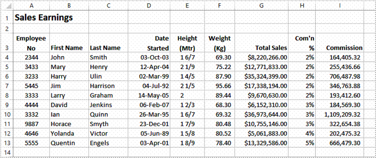
The following worksheet contains formatted numbers:
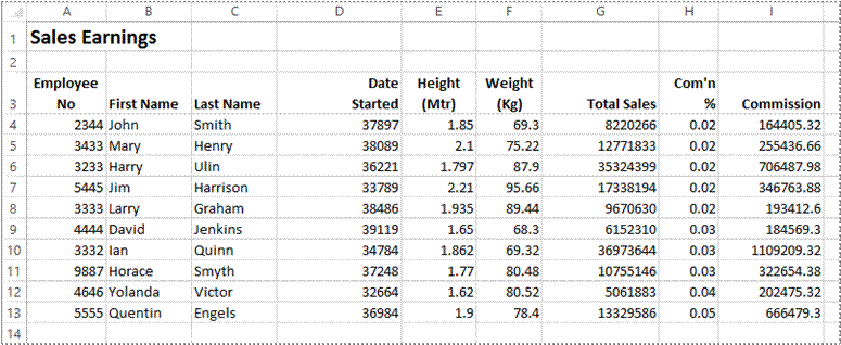
With the formatting removed from the numbers the worksheet looks as follows:
Formatting can also be applied as you type. For example, if you type 30/9/2020 Excel will place the number 44104 in the cell but will format this number as a date and show it as you typed it. There are also a range of number formatting options on the ribbon that allow you to apply formatting to numbers after they have been entered into a worksheet.
Source: https://www.sgul.ac.uk/about/our-professional-services/information-services/library/documents/training-manuals/Excel-Fundamentals-Manual.pdf
Web site to visit: https://www.sgul.ac.uk
Author of the text: indicated on the source document of the above text
If you are the author of the text above and you not agree to share your knowledge for teaching, research, scholarship (for fair use as indicated in the United States copyrigh low) please send us an e-mail and we will remove your text quickly. Fair use is a limitation and exception to the exclusive right granted by copyright law to the author of a creative work. In United States copyright law, fair use is a doctrine that permits limited use of copyrighted material without acquiring permission from the rights holders. Examples of fair use include commentary, search engines, criticism, news reporting, research, teaching, library archiving and scholarship. It provides for the legal, unlicensed citation or incorporation of copyrighted material in another author's work under a four-factor balancing test. (source: http://en.wikipedia.org/wiki/Fair_use)
The information of medicine and health contained in the site are of a general nature and purpose which is purely informative and for this reason may not replace in any case, the council of a doctor or a qualified entity legally to the profession.
The texts are the property of their respective authors and we thank them for giving us the opportunity to share for free to students, teachers and users of the Web their texts will used only for illustrative educational and scientific purposes only.
All the information in our site are given for nonprofit educational purposes