3.1 Introduction
A fluid is defined as a substance that deforms continuously when a shear stress is applied to it. Figure 3.1-1 shows the fluid motion when a force F is applied to a plate on top of the fluid causing the plate to move. As long as there is movement of the plate, the fluid continues to flow or deform since the fluid next to the plate is under the action of a shear stress equal to the force F divided by the surface area of the plate. When a fluid is at rest (no relative motion between the fluid elements), there can be no shear stress.
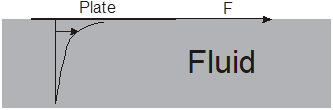
Figure 3.1-1 Fluid moves with the plate.
Both liquids and gases are fluids even though they are quite different at the molecular level. In liquids the molecules are held close together by significant attraction forces; in gases are relatively far apart and have very weak attraction forces. Figure 3.1-2 shows a PV diagram for water where the isotherms are plotted with the isotherm of highest temperature on the top. An isotherm is a curve that relates pressure to volume at a constant temperature. As temperature and pressure increase, the differences between liquid and gas become less and less, until the liquid and gas become identical at the critical point. For water the critical point occurs at 374.14oC and 22.09 MPa. Because of their closer molecular spacing, liquids normally have higher densities, viscosities, and other physical properties than gases.
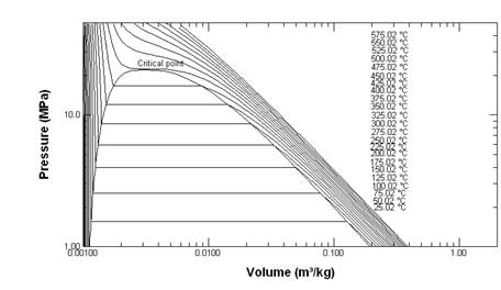
Figure 3.1-2 PV diagram for water.
3.2 Rheology
Rheologh is the study of the deformation and flow behavior of fluids. For a Newtonian fluid, we have a linear relationship between shear stress (t) and the shear rate (![]() ) or rate of shear strain.
) or rate of shear strain.
t = m![]() (3.2-1)
(3.2-1)
In this equation, the proportional constant m is called the viscosity of the fluid. The viscosity is the property of a fluid to resist the rate at which deformation takes place when the fluid is acted upon by a shear forces. As a property of the fluid, the viscosity depends upon the temperature, pressure, and composition of the fluid, but is independent of the shear rate. Most simple homogeneous liquids and gases are Newtonian fluid.
Figure 3.2-1 Deformation of a fluid element.
The rate of deformation of a fluid element for a simple one-dimensional flow is illustrated in Figure 3.2-1. The flow parallel to the x-axis will deform the element if the velocity at the top of the element is different than the velocity at the bottom. The shear rate at a point is defined as
![]() =
= ![]() =
= ![]()
![]()
![]() =
= ![]()
![]()
![]() = -
= - ![]()
![]()
For small angle q, arctan(q) = q, therefore
![]() = -
= - ![]()
![]() = -
= - ![]()
![]()
![]() =
= ![]() = -
= - ![]()
The shear stress for this simple flow is also the molecular momentum flux in the y-direction and is given as
tyx= - m![]() (3.2-2)
(3.2-2)
The subscript yx on tyx denotes the viscous flux of x momentum in the y direction. In this equation, the shear stress is defined to be the same as the momentum flux (tyx)mf. We may use equation (3.2-2) to obtain an expression for shear stress as a function of the fluid velocity and the system dimension. Consider the situation shown in Figure 3.2-2 where a fluid is contained between two large parallel plates both of area A. The plates are separated by a distance h. The system is initially at rest then a force F is suddenly applied to the lower plate to set the plate into motion in the x direction at a constant velocity V. Momentum is transferred from a region of higher velocity to a region of lower velocity. As time proceeds, momentum is transferred in the y direction to successive layers of fluid from the plate that is in motion in the x direction.
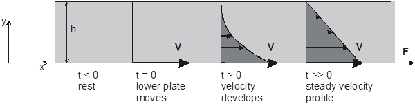
Figure 3.2-2 Velocity profile development for a flow between two parallel plates.
The velocity profile of the fluid between the parallel plates may be obtained by applying the momentum balance, which states that
Time rate of change |
rate of linear |
rate of linear |
sum of external |
Since the velocity in the x direction vx is dependent on the y direction, we choose the control volume CV to be ADy as shown in Figure 3.3-3.
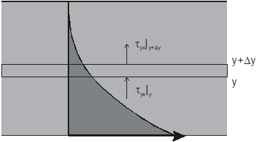
Figure 3.3-3 x-Momentum entering and leaving the CV = ADy
Applying the x-momentum balance on the CV yields
![]() ( ADyr vx) =
( ADyr vx) = ![]() A -
A - ![]() A
A
Dividing the equation by ADy and letting Dy ® 0, we obtain for constant physical properties
r![]() = -
= - ![]()
 = -
= - ![]() (3.2-3)
(3.2-3)
Substituting tyx= - m![]() into equation (3.2-3) yields a second order partial differential equation (PDE)
into equation (3.2-3) yields a second order partial differential equation (PDE)
r![]() = m
= m![]() Þ
Þ ![]() = n
= n![]() (3.2-4)
(3.2-4)
where n = m/r is the kinematic viscosity of the fluid. Equation (3.2-4) can be solved with the following initial and boundary conditions:
Initial condition: t = 0, vx = 0 (3.2-4a)
Boundary conditions: y = 0, vx = V and y = h, vx = 0 (3.2-4b)
Equation (3.2-4) with the auxiliary conditions (3.4-2a,b) can be solved by the separation of variables method with the following result
vx = V(1 - ![]() ) -
) - ![]()
![]() exp
exp![]() sin
sin![]()
The solution can also be expressed in dimensionless form with vx* = ![]() , y* =
, y* = ![]() , t* =
, t* = ![]()
vx* = 1 - y* - ![]()
![]() exp
exp![]() sin(np y*) (3.2-5)
sin(np y*) (3.2-5)
Table 3.2-1 lists the Matlab program to plot dimensionless velocity profiles at various dimensionless times. The results are shown in Figure 3.2-4.
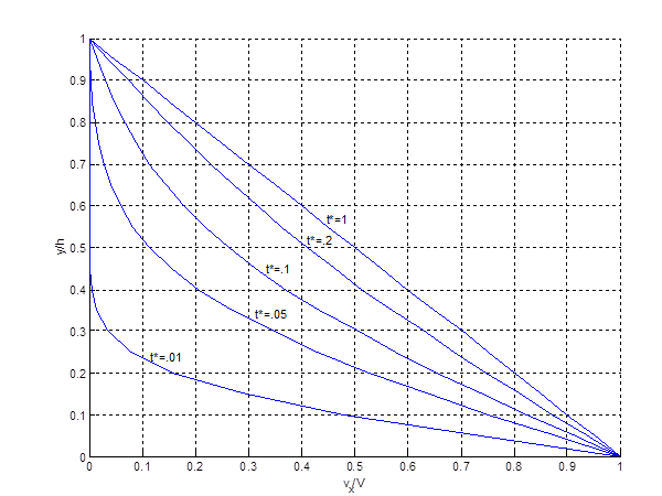
Figure 3.2-4 Dimensionless velocity profiles for flow between two parallel plates.
____ Table 3.2-1 Matlab program to plot vx* = 1 - y* - ![]()
![]() exp
exp![]() sin(np y*)___
sin(np y*)___
As time approaches infinity, the system reaches steady state and the summation terms in equation (3.2-5) become zero. The steady state velocity profile is then
vx* = 1 - y* (3.2-6)
The steady state solution can also be obtained directly from equation (3.2-4) by setting the temporal derivative equal to zeo.
![]() = 0 (3.2-7)
= 0 (3.2-7)
Integrating equation (3.2-7) twice, we obtain
vx = Ay + B
The two constants of integration are evaluated from the boundary conditions:
y = 0, vx = V and y = h, vx = 0
Therefore B = V and A = - V/h
Hence vx = V(1- y/h) Þ vx* = 1 - y*
The shear rate at any position y in the fluid is given as ![]() = -
= - ![]() =
= ![]()
The force to pull the lower plate at velocity V can be evaluated: F = A![]() = Am
= Am![]()
Fluids are classified as Newtonian or non-Newtonian, depending upon the relation between shear stress and shear rate. In Newtonian fluids the relation is linear while in non-Newtonian fluids, the shear stress is not a linear function of shear rate as shown in Figure 3.2-5.
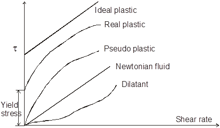
Figure 3.2-5 Behaviors of Newtonian and non-Newtonian fluids.
The slope of the Newtonian fluid line is the viscosity. For the non-Newtonian fluids, the slope is not constant therefore its value at a given shear rate is called the apparent viscosity. The apparent viscosity of a dilatant fluid increases with shear rate while the apparent viscosity of a pseudo platic decreases with shear rate. The ideal or Bingham plastic has a linear shear stress-shear rate relation for stresses greater than the yield stress. Real plastic or Carson fluid also flows with stresses greater than the yield stress. The apparent viscosity however decreases with shear rate and at some point the Carson fluid behaves as a Newtonian fluid. Heterogeneous fluids that contain a particulate phase that forms aggregates at low rates of shear require a yield stress.
Blood is a heterogeneous fluid with the particulates consisting primarily of the red blood cells. Therefore blood follows the curve shown for real plastic. At low shear rates, red blood cells clump together to form aggregates. This behavior results in high value of apparent viscosity. However, at shear rate higher than 100/s, red blood cells do not clump together, therefore blood behaves as a Newtonian fluid with an apparent viscosity of about 3 cP. The properties of blood change rapidly if removed from the system and so it is extremely difficult to perform experiments on it under laboratory conditions.
3.3 Fully Developed Laminar Flow in Tube
We want to develop a relationship for shear stress-shear rate given volume flow rate Q and pressure drop DP across the horizontal tube as shown in Figure 3.3-1. We use cylindrical coordinates with the following assumptions: the length of the tube (L) is much larger than the tube radius (R) (i.e. L/R > 100) to eliminate entrance effect; steady incompressible and isothermal flow; one-dimensional flow in the z direction only, therefore vz = vz(r); and no-slip boundary condition at the wall.
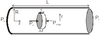
Figure 3.3-1 Forces acting on a cylindrical fluid element within a tubey.
Consider the control volume pr2Dz shown in Figure 3.5-1. For steady flow, the summation of the viscous and pressure forces acting on the control volume must be equal to zero.
P|zpr2 - trz2prDz - P|z+Dzpr2 = 0
Dividing the equation by the control volume yields
- ![]() =
= ![]() trz
trz
In the limit when Dz ® 0, we obtain the differential equation for the shear stress distribution
- ![]() =
= ![]() trz (3.3-1)
trz (3.3-1)
Since trz = - m![]() , the right hand side of equation (3.3-1) is a function of r only and the left hand side of equation (3.3-1) is a function of z only. They both must be equal to a constant
, the right hand side of equation (3.3-1) is a function of r only and the left hand side of equation (3.3-1) is a function of z only. They both must be equal to a constant
- ![]() =
= ![]() trz =
trz = ![]()
The equation is rearranged to
trz = - ![]()
![]() =
= ![]() (3.3-2)
(3.3-2)
The shear stress vanishes at the centerline of the tube and achieves its highest value, tw, at the wall.
tw = trz|r=R = - ![]()
![]() =
= ![]() (3.3-3)
(3.3-3)
Equations (3.3-2) and (3.3-3) are valid for both Newtonian and non-Newtonian fluids since we has not specified a relationship between the shear stress and shear rate. Solving equations (3.3-2) and (3.3-3) for ![]() yields
yields
- ![]() =
= ![]() trz =
trz = ![]() tw
tw
Therefore trz = ![]() tw =
tw = ![]() (3.3-4)
(3.3-4)
If ![]() = m = constant, the fluid is a Newtonian fluid and m is called the viscosity. If
= m = constant, the fluid is a Newtonian fluid and m is called the viscosity. If ![]() = h ¹ constant, the fluid is a non-Newtonian fluid and h is called the apparent viscosity. We will follow different procedures to determine a relationship between shear stress and shear rate depending on whether or not
= h ¹ constant, the fluid is a non-Newtonian fluid and h is called the apparent viscosity. We will follow different procedures to determine a relationship between shear stress and shear rate depending on whether or not![]() and trz are known directly.
and trz are known directly.
A)![]() and trz are not known directly
and trz are not known directly
We want to find a general relationship between the shear rate and some function of the shear stress in terms of the measurable quantities Qmeas., Po - PL, L, and R. That is:
![]() = -
= - ![]() =
= ![]() (trz) (3.3-5)
(trz) (3.3-5)
We can follow the following procedures to obtain a relationship between the shear rate ![]() and shear stress trz.
and shear stress trz.
1) We calculate the volumetric flow rate from the axial velocity profile as follows.
Qcal = 2p![]() rdr
rdr
2) We express Qcal in terms of shear rate using integration by part.
d(uv) = vdu + udv Þ ![]() du =
du = ![]() -
- ![]() dv
dv
Let v = vz(r) Þ dv = dvz(r)
du = rdr Þ u = ![]() r2
r2
Therefore Qcal = 2p![]() r2
r2![]() - 2p
- 2p![]()
![]() dr = - p
dr = - p![]()
![]() dr
dr
3) Next, we change the integration variable from r to trz using equation (3.3-4)
trz = ![]() tw Þ r =
tw Þ r = ![]() trzÞ dr =
trzÞ dr = ![]() dtrz
dtrz
Qcal = p![]()
![]()
![]()
![]() dtrz , (Note:
dtrz , (Note: ![]() = -
= - ![]() )
)
Qcal = ![]()
![]()
![]() dtrz (3.3-6)
dtrz (3.3-6)
4) We then assume a relationship between ![]() and trz (for example
and trz (for example ![]() =
= ![]() ).
).
Equation (3.3-6) is then integrated to obtain Qcal. We will accept the assumed expression between ![]() and trzif Qcal » Qmeas. Otherwise step (4) is repeated.
and trzif Qcal » Qmeas. Otherwise step (4) is repeated.
B)![]() and trz are known directly
and trz are known directly
The shear stress and shear rate can be determined using a cup-and-bob or Couette viscometer. As the name implies, the Couette viscometer consists of two concentric cylinders as shown in Figure 3.3-2. The fluid is in the annular gap between the outer cylinder (cup) and the inner cylinder (bob).
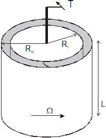
Figure 3.3-2 Couette viscometer.
The outer cylinder is rotated at a fixed angular velocity (W). The shearing force is transmitted to the fluid, causing it to deform or flow. The inner cylinder is kept stationary by a torque (T) that can be measured by a torsion spring. The shear stress at any position r within the gap (Ri £ r £ Ro) is determined by a balance of moments on a cylindrical surface 2prL
T = trq(2prL)r
Solving for the shear stress, we have
trq = ![]() (3.3-7)
(3.3-7)
Setting r = Ri gives the stress on the bob surface (ti), and setting r = Ro gives the stress on the cub surface (to). If the gap is small [i.e., (Ro - Ri)/Ro £ 0.02], the flow in the annular gap can be approximated by the flow between two parallel plates. In this case, an average shear stress should be used
trq = ![]() »
» ![]() where
where ![]() = (Ri + Ro)/2 (3.3-8)
= (Ri + Ro)/2 (3.3-8)
The average shear rate is given by
![]() =
= ![]() »
» ![]() =
= ![]() =
= ![]() (3.3-9)
(3.3-9)
Equations (3.3-8, 9) provide the experimental values for the shear stress and the shear rate that can be fitted by a non-Newtonian fluid model.
Example 3.3-1.0 ----------------------------------------------------------------------------------
The viscosity of a fluid sample is measured in a cup-and-bob viscometer. The bob is 15 cm long with a diameter of 9.8, and the cup has a diameter of 10 cm. The cup rotates, and the torque is measured on the bob. The following data were obtained:
W(rpm) |
2 |
4 |
10 |
20 |
40 |
T (dyn×cm) |
3.6´105 |
3.8´105 |
4.4´105 |
5.4´105 |
7.4´105 |
(a) Determine the viscosity of the sample.
(b) Fit the data with the following model equations
t = to + m¥![]() (Bingham Plastic Model)
(Bingham Plastic Model)
and t = m![]() n (Power Law Model)
n (Power Law Model)
(c) Determine the viscosity of this sample at a cup speed of 100 rpm in the viscometer using the above models.
Solution ------------------------------------------------------------------------------------------
Since (Ro - Ri)/Ro = (10 - 9.8)/10 = 0.02, we can use the equation (3.3-8, 9) to determine the shear stress and the shear rate
trq = ![]() , and
, and ![]() =
= ![]()
The apparent viscosity h is determined from
h = ![]()
Table 3.3-1 lists the results from the calculation. Table 3.3-2 lists the Matlab program to fit data with the Bingham plastic and power law model.
Table 3.3-1 Fluid apparent viscosity at different shear rates
W(rpm) |
T (dyn×cm) |
|
trq(dyne/cm2) |
h(Poise = g/cm×s) |
2 |
360000 |
10.5 |
156 |
14.89 |
For the Bingham plastic model, we obtain
t (dyne/cm2) = to + m¥![]() = 147 + 0.827
= 147 + 0.827![]() (1/s)
(1/s)
For the power law model, we obtain
t(dyne/cm2) = m![]() n = 83.2
n = 83.2![]() 0.234
0.234
At 100 rpm or ![]() = 524 s-1, for the Bingham plastic model
= 524 s-1, for the Bingham plastic model
t = 147 + 0.827´524 = 580 dyne/cm2
h = 580/524 = 1.11 g/cm×s
For the power law model
h = ![]() = 83.2
= 83.2![]() 0.234-1 = 0.69 g/cm×s
0.234-1 = 0.69 g/cm×s
______ Table 3.3-2 Matlab program to fit shear stress and shear rate data ______
>> e3d1
shear_rate =
10.4720 20.9440 52.3599 104.7198 209.4395
stress =
155.8910 164.5516 190.5334 233.8365 320.4426
vis =
14.8865 7.8568 3.6389 2.2330 1.5300
tao =
147.2304
vis_inf =
0.8270
n =
0.2337
m =
83.1932
Correlation coefficient for Bingham plastic = 1.0000
Correlation coefficient for Power law = 0.9938
A crude measure of the how well the data is fitted by an expression is given by the correlation coefficient r, which is defined as
r = 
In this expression St = ![]() is the spread of the data around the mean
is the spread of the data around the mean ![]() of the dependent variable and S =
of the dependent variable and S = ![]() is the sum of the square of the difference between the data (Yi) and the calculated value (yi).
is the sum of the square of the difference between the data (Yi) and the calculated value (yi).
Figure 3.3-3 shows a plot of viscosity versus flow rate for the Bingham plastic and the Power law models. The Bingham plastic model fits the data better as evident by its higher correlation coefficient (1.0) in comparison with that (0.9938) of the Power law model.
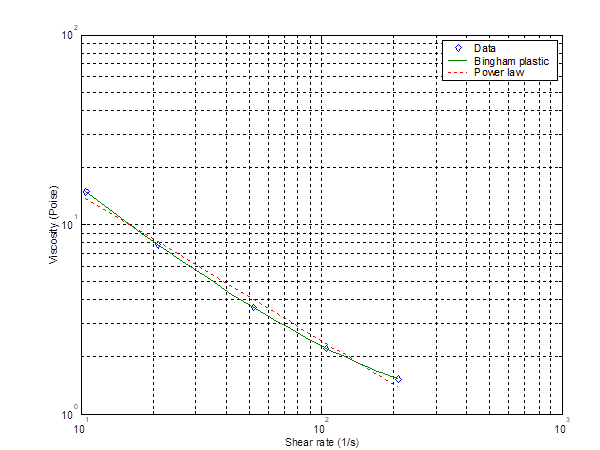
Figure 3.3-3 Behavior of non-Newtonian fluid.
---------------------------------------------------------------------------------------------------
3.4 The Hagan-Poiseuille Equation
We now consider the case of a Newtonian fluid flowing through a capillary. The shear rate-shear stress relation ![]() (trz) =
(trz) = ![]() is substituted into equation (3.3-6) to obtain
is substituted into equation (3.3-6) to obtain
Q = ![]()
![]() dtrz =
dtrz = ![]()
![]() =
= ![]()
![]()
Q = ![]() tw =
tw = ![]()
![]() =
= ![]()
The velocity profile inside the capillary can also be obtained by integrating equation (3.3-2)
trz = - m![]() =
= ![]() (3.3-2)
(3.3-2)
trz = - m![]() =
= ![]() (3.3-2)
(3.3-2)
![]() = -
= - ![]()
![]()
vz = ![]()

Example 3.4-1. 1 ----------------------------------------------------------------------------------
You are asked to measure the viscosity of an emulsion, so you use a tube flow viscometer similar to that shown below, with the container open to the atmosphere.
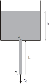
The length of the tube is 10 cm, its diameter is 2 mm, and the diameter of the container is 3 in. When the level of the sample is 10 cm above the bottom of the container the emulsion drains through the tube at a rate of 12 cm3/min, and when the level is 20 cm the flow rate is 30 cm3/min. The emulsion density is 1.3 g/cm3. What can you tell from the data about the viscous properties of the emulsion?
Solution ------------------------------------------------------------------------------------------
Equation (3.3-3) provides a relation between the wall shear stress and the pressure drop across the tube
tw = trz|r=R = - ![]()
![]() =
= ![]() (3.3-3)
(3.3-3)
This equation is valid for any Newtonian or non-Newtonian fluid. Po is essentially the pressure at the bottom of the container and PL is the ambient pressure Patm. Therefore
Po - PL = rgh
The wall shear stress is then given by
tw = ![]()
where d is the inside diameter of the tube.
When h = 10 cm, tw1 = ![]() = 63.7 dyne/cm2
= 63.7 dyne/cm2
When h = 20 cm, tw2 = ![]() = 127.4 dyne/cm2
= 127.4 dyne/cm2
If the fluid is a Newtonian fluid then
Q = ![]() tw
tw
so that ![]() =
= ![]() = 2
= 2
From experimental data
 =
= ![]() = 2.5
= 2.5
Therefore the viscosity at high shear rate is smaller than that at lower shear rate. The emulsion is a shear thinning liquid.
1 Darby, R., Chemical Engineering Fluid Mechanics, Marcel Dekker, 2001, p. 80
Source: https://www.cpp.edu/~tknguyen/che311/notes/Chapter3.doc
Web site to visit: https://www.cpp.edu
Author of the text: indicated on the source document of the above text
If you are the author of the text above and you not agree to share your knowledge for teaching, research, scholarship (for fair use as indicated in the United States copyrigh low) please send us an e-mail and we will remove your text quickly. Fair use is a limitation and exception to the exclusive right granted by copyright law to the author of a creative work. In United States copyright law, fair use is a doctrine that permits limited use of copyrighted material without acquiring permission from the rights holders. Examples of fair use include commentary, search engines, criticism, news reporting, research, teaching, library archiving and scholarship. It provides for the legal, unlicensed citation or incorporation of copyrighted material in another author's work under a four-factor balancing test. (source: http://en.wikipedia.org/wiki/Fair_use)
The information of medicine and health contained in the site are of a general nature and purpose which is purely informative and for this reason may not replace in any case, the council of a doctor or a qualified entity legally to the profession.
The texts are the property of their respective authors and we thank them for giving us the opportunity to share for free to students, teachers and users of the Web their texts will used only for illustrative educational and scientific purposes only.
All the information in our site are given for nonprofit educational purposes