Static Loading

Chapter 5           Failures Resulting from Static Loading

• A static (steady) load is a stationary force or couple (applied to a member) that does not change in magnitude, point of application, and direction.
• A static load can produce axial tension or compression, a shear load, a bending load, a torsional load, or any combination of these.
• We consider the relations between strength and static loading make decisions concerning material and its treatment, fabrication, and geometry for satisfying the requirements of functionality, safety, reliability, competitiveness, usability, manufacturability, and marketability.
• Stress is dependent on the load characteristics.
• Strength is an inherent property of the material.
• Factor of safety =  Strength / Stress = S / σ
• Factor of safety depends on
• type of material
• how controllable are environment conditions
• type of loading and the degree of certainty with which the stresses are calculated
• type of application
• Failure can mean a part
• has separated into two or more pieces; (brittle)
• has become permanently distorted, thus ruining its geometry; (ductile)
• has had its reliability reduced; or
• has had its function compromised.
• A designer speaking of failure can mean any or all of these possibilities.
• It is by thinking in terms of avoiding failure that successful designs are achieved.

 

• Next are photographs of several failed parts:

Failure of truck driveshaft spline due to corrosion fatigue

 

Impact failure of a lawn-mower
blade driver hub. The blade impacted a surveying pipe marker.

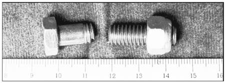
Failure of an overhead-pulley retaining bolt on a weightlifting machine. A manufacturing error caused a gap that forced the bolt to take the entire moment load.

 

Valve-spring failure caused by spring surge in an oversped engine. The fractures exhibit the classic 45° shear failure.

 

•   Static Strength
• Ideally, in designing any machine element, the engineer should have available the results of a great many strength tests of the particular material chosen.
• These tests should be made on specimens having the load conditions, same heat treatment, surface finish, and size as the element the engineer proposes to design.
• The cost of gathering such extensive data prior to design is justified if failure of the part may endanger human life or if the part is manufactured in sufficiently large quantities.

 

• You can now appreciate the following four design categories:
• Failure of the part would endanger human life; consequently, an elaborate testing program is justified.
• The part is made in large enough quantities that a moderate series of tests is feasible.
• The part is made in such small quantities that testing is not justified at all; or the design must be completed so rapidly that there is not enough time for testing.
• The part has already been designed, manufactured, and tested and found to be unsatisfactory. Analysis is required to understand why the part is unsatisfactory and what to do to improve it.
• More often it is necessary to design using only published values of yield strength, ultimate strength, percentage reduction in area, and percentage elongation.
• How can one use such meager data to design against both static and dynamic loads, two- and three-dimensional stress states, high and low temperatures, and very large and very small parts? These and similar questions will be addressed in this chapter and those to follow.
•   Stress Concentration
• Recall from section 3.13, there is a localized increase of stress near discontinuities
• A theoretical (geometric) stress-concentration factor Kt or Kts is used to relate the actual maximum stress at the discontinuity to the nominal stress:

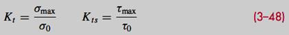
• The nominal stress σ0 or τ0 is the stress calculated by using the elementary stress equations and the net cross section.

 

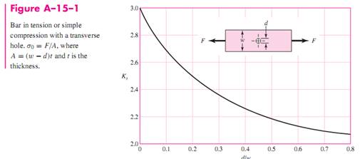
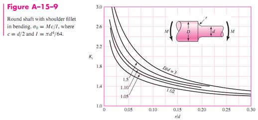
• Graphs available for standard configurations
• See Appendix A–15 and A–16 for common examples
• Many more in R.E. Peterson’s Stress-Concentration Factors
• Note the trend for higher Kt  at sharper discontinuity radius, and at greater disruption

 

•   Failure Theories
• Unfortunately, there is no universal theory of failure. Instead, over the years several hypotheses have been formulated and tested, leading to today’s accepted practices.
• Being accepted, we will characterize these “practices” as theories as most designers do.

• Structural metal behavior is typically classified as being ductile or brittle

• Ductile materials are normally classified such that:
• Strain at failure is εf ≥ 0.05 or percent elongation is greater than 5%
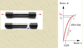
• They typically have well defined (identifiable) yield strength, Sy.
• Their tensile and compressive yield strengths are almost equal (Syt ≈ Syc = Sy ).
• Slow large amount of strain than brittle materials

 

• Brittle materials, εf < 0.05, do not exhibit identifiable yield strength, and are typically classified by ultimate tensile and compressive strengths, Sut and Suc, respectively.
• Strain at failure is εf < 0.05 or percent elongation is less than 5%.
• Do not have identifiable yield strength; rather, they fail by brittle fracture. Typically classified by ultimate tensile and compressive strengths, Sut and Suc, respectively.
• The compressive strength of a typical brittle material is significantly higher than its tensile strength, Suc >> Sut .
• Show smaller amount of strain than ductile materials

In static loading, stress-concentration factors are applied as follows.
In ductile materials, the stress-concentration factor is not usually applied to predict the critical stress, because plastic strain in the region of the stress is localized and has a strengthening effect.
In brittle materials, the geometric stress-concentration factor Kt is applied to the nominal stress before comparing it with strength.
For dynamic loading, the stress concentration effect is significant for both ductile and brittle materials and must always be taken into account (see Sec. 6–10).

• Theories have been developed for the static failure of metals based upon the two classes of material failure:
• Ductile metals à yield
• Brittle metals  à fracture

Thus separate failure theories exit for ductile and brittle metals:

• Ductile materials (yield criteria)
• Maximum shear stress (MSS), Sec. 5–4
• Distortion energy (DE), Sec. 5–5
• Ductile Coulomb-Mohr (DCM), Sec. 5–6

• Brittle materials (fracture criteria)
• Maximum normal stress (MNS), Sec. 5–8
• Brittle Coulomb-Mohr (BCM), Sec. 5–9
• Modified Mohr (MM), Sec. 5–9

 

• These theories have grown out of hypotheses and experimental data in the following manner:

1.  Experimental failure data is first collected through tensile tests.
2.  The state of stress is correlated to the experimental data using Mohr’s circle plots.
3.  A failure theory is developed from a concept of the responsible failure mechanism.
4.  A design envelope is established based upon the theoretical and empirical design
     equations.

1. Tensile Test

We will first review the acquisition and correlation of tensile test data to failure theory.
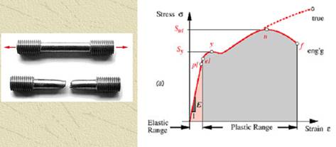
Recalling the standarized tensile test:
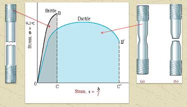
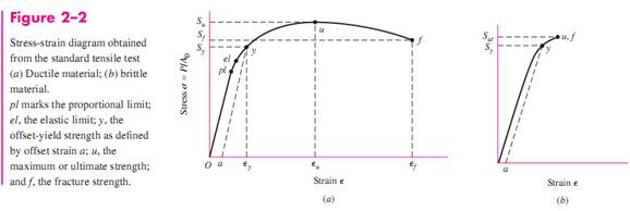
Stress-strain curves for ductile materials

Stress-strain curves for brittle materials

From chapter 2

2. Correlation of State of Stress with Test Data

For design, we need to relate the expected state of stress to the actual state of stress and thus, the material strength, as determined through the tensile test. We accomplish this by applying principal stresses since they characterize a state of stress independent of the original coordinate system.

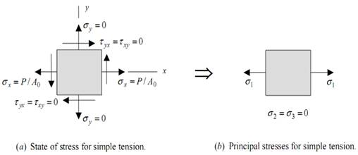
Correlation of state of stress with principal stresses for simple tension

Since tensile test generates a uniaxial state of stress, the principal stresses can be defined

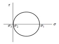
When plotted on a Mohr's circle diagram, these stress values look like a single circle passing through the origin where σ2 is coincident with σ3. There are still three circles. Two circles on the top of each other (σ1, σ2) and (σ1, σ3). Third circle degenerates a point circle (σ2, σ3)

Fig. 1 Mohr's Circle for Simple Tension
Note
Recall that in plotting Mohr’s circles for three-dimensional stress (after solving Eq. 3.15), the principal normal stresses are ordered so that σ1 ≥ σ2 ≥ σ3. See figure shown.

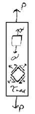
•   Maximum-Shear-Stress Theory for Ductile Materials
• Theory:

 “A mechanical part subject to any combination of loads will yield whenever the maximum shear stress (τmax ) in any stress element equals or exceeds the maximum shear stress in a tension-test specimen of the same material when that specimen begins to yield”

• The MSS theory is also referred to as the Tresca or Guest theory.
• Recall that for simple tensile stress,  σ = P/A, and the maximum shear stress occurs on a surface 45° from the tensile surface with a magnitude of τmax = σ/2 (see Fig. 1 above).
• So the maximum shear stress at yield is τmax = Sy /2.
• For a general state of stress, three principal stresses can be determined and ordered such that σ1 ≥ σ2 ≥ σ3. The maximum shear stress is then τmax = (σ1 − σ3)/2 (see above).
• Thus, for a general state of stress, the maximum-shear-stress theory predicts yielding when

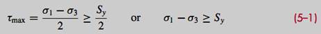
• Note that this implies that the yield strength in shear is given by

which, as will be seen later, is about 15 percent low (conservative).

• Could restate the theory as follows:

Yielding begins when the maximum shear stress in a stress element exceeds Sy/2.

• For design purposes, Eq. (5–1) can be modified to incorporate a factor of safety, n:

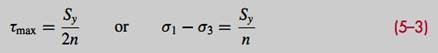
• Or solving for factor of safety                          
• For plane stress, we first label the principal stresses given by Eq. (3–13) as σA and σB, and then order them with the zero principal stress according to the convention σ1 ≥ σ2 ≥ σ3.
• Assuming that σA ≥ σB, there are three cases to consider when using Eq. (5–1) for plane stress:

 

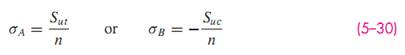
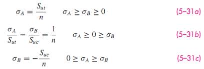
Case 1: σA ≥ σB ≥ 0.
For this case, σ1 = σA and σ3 = 0. Equation (5–1) reduces to a yield condition of

Case 2: σA ≥ 0 ≥ σB .
For this case, σ1 = σA and σ3 = σB , and Eq. (5–1) becomes

Case 3: 0 ≥ σA ≥ σB.
For this case, σ1 = 0 and σ3 = σB , and Eq. (5–1) gives

• Equations (5–4) to (5–6) are represented in Fig. 5–7 by the three lines indicated in the σA, σB plane. The remaining unmarked lines are cases for σB ≥ σA, which completes the stress yield envelope but are not normally used.
• The maximum-shear-stress theory predicts yield if a stress state is outside the shaded region bordered by the stress yield envelope. Inside envelope is predicted safe zone.

• In Fig. 5–7, suppose point a represents the stress state of a critical stress element of a member. If the load is increased, it is typical to assume that the principal stresses will increase proportionally along the line from the origin through point a. Such a load line is shown. If the stress situation increases along the load line until it crosses the stress failure envelope, such as at point b, the MSS theory predicts that the stress element will yield. The factor of safety guarding against yield at point a is given by the ratio of strength (distance to failure at point b) to stress (distance to stress at point a), that is n = Ob/Oa.

Shown is a comparison to experimental data. Envelope is conservative in all quadrants.
Commonly used for design situations

 

 

 

•    Distortion-Energy Theory for Ductile Materials
• The distortion-energy (DE) theory originated from the observation that ductile materials stressed hydrostatically (equal principal stresses) exhibited yield strengths greatly in excess of the values given by the simple tension test.
• Therefore it was postulated that yielding was not a simple tensile or compressive phenomenon at all, but, rather, that it was related somehow to the angular distortion of the stressed element.
• Theory:  “Yielding occurs when the distortion strain energy per unit volume reaches or exceeds the distortion strain energy per unit volume for yield in simple tension or compression of the same material”.
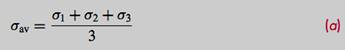
• From Fig. 5–8a, the unit volume subjected to any 3-D stress state designated by the stresses σ1, σ2, and σ3. Fig. 5–8b is one of hydrostatic normal stresses due to the stresses σav acting in each of the same principal directions as in (a). The formula for σav is simply

• Thus the element in Fig. 5–8b undergoes pure volume change, that is, no angular distortion. Hence, in Fig. 5–8c, this element is subjected to pure angular distortion, that is, no volume change.

• The strain energy per unit volume for simple tension is
• For the element of Fig. 5–8a the strain energy per unit volume is 

                  (a1)

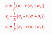
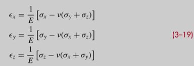
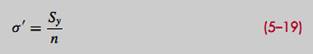
• Use Eq. (3–19) to substitute for the principal strains in Eq. (a1)

• Then the total strain energy per unit volume subjected to three principal stresses is :

• Strain energy for producing only volume change (uv) is obtained by substituting σavfor σ1, σ2, and σ3

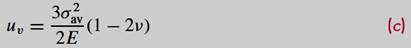
• Substituting σav from Eq. (a) into Eq (c)

• Obtain distortion energy by subtracting volume changing energy Eq. (5–7)  from total strain energy Eq. (b):

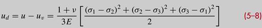
Note that the distortion energy is zero if σ1 = σ2 = σ3.

• For the simple tensile test, at yield, σ1 = Sy and σ2 = σ3 = 0, and from Eq. (5–8) the distortion energy is

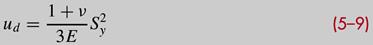
• DE theory predicts failure when distortion energy, Eq. (5–8), exceeds distortion energy of tension test specimen, Eq. (5–9)

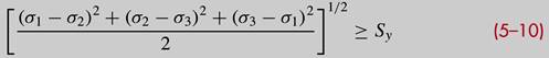
• For a simple tension σ , then yield would occur when σ ≥ Sy . Thus, the left of Eq. (5–10) can be thought of as a single, equivalent, or effective stress for the entire general state of stress given by σ1,σ2, and σ3. This effective stress is called the von Mises stress, σ', named after Dr. R. von Mises. Thus Eq. (5–10), for yield, can be written as

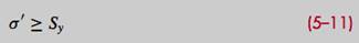
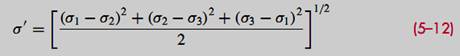
where the von Mises stress is

• Eq. (5-11) equation can be expressed as a design equation by

• For plane stress, the von Mises stress can be represented by the principal stresses σA , σB , and zero. Then from Eq. (5–12), we get

Equation (5–13) is a rotated ellipse in the σA , σB plane, as shown in Fig. 5–9 with σ' = Sy . The dotted lines in the figure represent the MSS theory, which can be seen to be more restrictive, hence, more conservative.

• Using xyz components of three-dimensional stress, the von Mises stress can be written as

and for plane stress,

• The distortion-energy theory is also called: (give the same results)

• The von Mises or von Mises–Hencky theory
• The shear-energy theory
• The octahedral-shear-stress theory

• Understanding octahedral shear stress will explain why the MSS is conservative. Octahedral stresses allow representation of any stress situation with a set of normal and shear stresses.
• Consider an isolated element in which the normal stresses on each surface are equal to the hydrostatic stress σav.
• There are eight surfaces symmetric to the principal directions that contain that stress.

This forms an octahedron as shown in the figure below.

 
  

 

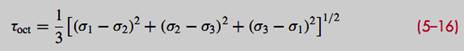
• The shear stresses on these surfaces are equal and are called the octahedral shear stresses (Fig. 5–10 has only one of the octahedral surfaces labeled). Through coordinate transformations the octahedral shear stress is given by

• Under the name of the octahedral-shear-stress theory: ” failure is assumed to occur whenever the octahedral shear stress for any stress state equals or exceeds the octahedral shear stress for the simple tension-test specimen at failure”.
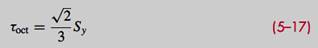
• As before, from simple tensile test results, yield occurs when σ1 = Sy and σ2 = σ3 = 0. From Eq. (5–16) the octahedral shear stress under this condition is

• When, for the general stress case, Eq. (5–16) is equal or greater than Eq. (5–17), yield is predicted. This reduces to

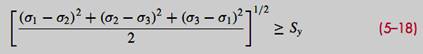
which is identical to Eq. (5–10), verifying that the maximum-octahedral-shear-stress theory is equivalent to the distortion-energy theory.

• The model for the MSS theory ignores the contribution of the normal stresses on the 45° surfaces of the tensile specimen. However, these stresses are P/2A, and not the hydrostatic stresses which are P/3A. Herein lies the difference between the MSS and DE theories.
• The distortion-energy theory predicts no failure under hydrostatic stress and agrees well with all data for ductile behavior.

Hence, it is the most widely used theory for ductile materials and is recommended for design problems unless otherwise specified.

• One final note concerns the shear yield strength. Consider a case of pure shear τxy , where for plane stress σx = σy = 0. For yield, Eq. (5–11) with Eq. (5–15) gives

 

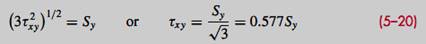
Thus, the shear yield strength predicted by the distortion-energy theory

which as stated earlier (Eq. 5.2), is about 15 percent greater than the 0.5 Sy predicted by the MSS theory.

• For pure shear τxy , the principal stresses from Eq. (3–13) are σA =−σB = τ .

The load line for this case is in the third quadrant at an angle of 45o from the σA, σB axes shown in Fig. 5–9.

Example 5-1 (see textbook)
 

•   Coulomb-Mohr Theory for Ductile Materials
• Not all materials have compressive strengths equal to their corresponding tensile values. For example, the Syc ~= 0.5 Syt for magnesium alloys;

      the Suc ~= (3-4) Sut for gray cast irons.
In this section we are interested in such materials.

• The idea of Mohr is based on three “simple” tests: tension, compression, and shear, to yielding if the material can yield, or to rupture. It is easier to define shear yield strength as Ssy than it is to test for it.

 

 

 

• Mohr’s hypothesis was to use the results of tensile, compressive, and torsional shear tests to construct the three circles of Fig. 5–12 defining a failure envelope tangent to the three circles, depicted as curve ABCDE in the figure.
• A variation of Mohr’s theory, called the Coulomb-Mohr theory or the internal-friction theory, assumes that the boundary BCD in Fig. 5–12 is straight. With this assumption only the tensile and compressive strengths are necessary.

• Consider the order of the principal stresses σ1 ≥ σ2 ≥ σ3. The largest circle connects σ1 and σ3, as shown above. The centers of the circles in Fig. 5–13 are C1 , C2 , and C3 .

Failure will occur if Mohr’s circle (3-D) describing a state of describing a state of stress in a body grows until it becomes tangent to the failure envelope.

 

• Triangles OBi Ci  are similar, therefore

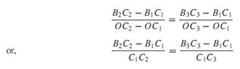
where B1C1 = St /2, B2C2 = (σ1 − σ3)/2, and B3C3 = Sc/2, are the radii of the right, center, and left circles, respectively. The distance from the origin to C1 is St /2, to C3 is Sc/2, and to C2 (in the positive σ direction) is (σ1 + σ3)/2. Thus

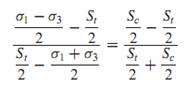
Canceling the 2 in each term, cross-multiplying, and simplifying reduces this equation to

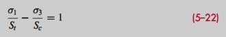
• For plane stress, when the two nonzero principal stresses are σA ≥ σB , we have a situation similar to the three cases given for the MSS theory, Eqs. (5–4) to (5–6).

That is, the failure conditions are
Case 1: σA ≥ σB ≥ 0.
For this case, σ1 = σA and σ3 = 0. Equation (5–22) reduces to

Case 2: σA ≥ 0 ≥ σB .
For this case, σ1 = σA and σ3 = σB , and Eq. (5–22) becomes

Case 3: 0 ≥ σA ≥ σB.
For this case, σ1 = 0 and σ3 = σB , and Eq. (5–22) gives

• A plot of these cases, together with the normally unused cases corresponding to σB ≥ σA, is shown in Fig. 5–14.

 

 

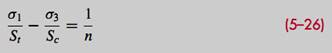
• As a design equation, Eq. (5–22) can be written as

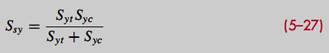
• Since for the Coulomb-Mohr theory we do not need the torsional shear strength circle we can deduce it from Eq. (5–22). For pure shear τ, σ1 =−σ3 = τ . The torsional yield strength occurs when τmax = Ssy . Substituting σ1 =−σ3 = Ssy into Eq. (5–22) and simplifying gives

Example 5-2 (see textbook)

•   Failure of Ductile Materials Summary
• To help decide on appropriate and workable theories of failure, data collected (by Marin and Mann) from many sources. See Fig. 5-15.  
• Fig.  5–15 shows that either the maximum-shear-stress theory or the distortion-energy theory is acceptable for design and analysis of a ductile material.

• The selection of one or the other of these two theories is something that you, the engineer, must decide.
• For design purposes the maximum-shear-stress theory is easy, quick to use, and conservative.
• If the problem is to learn why a part failed, then the distortion-energy theory may be the best to use; Fig. 5–15 shows that the plot of the distortion-energy theory passes closer to the central area of the data points, and thus is generally a better predictor of failure.
• For ductile materials with unequal yield strengths, Syt in tension and Syc in compression, the Mohr theory is the best available. However, the theory requires the results from three separate modes of tests, graphical construction of the failure locus, and fitting the largest Mohr’s circle to the failure locus.
• The alternative to this is to use the Coulomb-Mohr theory, which requires only the tensile and compressive yield strengths and is easily dealt with in equation form.

Examples 5-3 and 5-4 (see textbook)

 

 

 

 

 

•   Maximum-Normal-Stress Theory for Brittle Materials
• The maximum-normal-stress (MNS) theory states that failure occurs whenever one of the three principal stresses equals or exceeds the strength.
• Recall that principle stresses for a general stress state in ordered form are σ1 ≥ σ2 ≥ σ3. This theory then predicts that failure occurs whenever

where Sut and Suc are the ultimate tensile and compressive strengths, respectively, given as positive quantities.

• For plane stress, with the principal stresses given by Eq. (3–13), with σA ≥ σB, Eq. (5–28) can be written as

which is plotted in Fig. 5–18.

• As before, the failure criteria equations can be converted to design equations. We can consider two sets of equations where σA ≥ σB as

As will be seen later, the maximum-normal-stress theory is not very good at predicting failure in the fourth quadrant of the σA, σB plane. Thus, we will not recommend the theory for use. It has been included here mainly for historical reasons.

•   Modifications of the Mohr Theory for Brittle Materials
• Two modifications of the Mohr theory for brittle materials: the Brittle-Coulomb-Mohr (BCM) theory and the modified Mohr (MM) theory; introduced for plane stress.
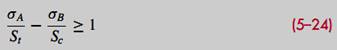
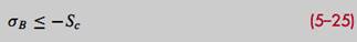
• The Coulomb-Mohr theory (Sec. 5–6: Eqns. (5–23) to (5–25)). Written as design equations for a brittle material, they are:

Brittle-Coulomb-Mohr

• On the basis of observed data for the fourth quadrant, the modified Mohr theory expands the fourth quadrant with the solid lines shown in the second and fourth quadrants of Fig. 5–19.

Data are still outside this extended region. The straight line introduced by the modified Mohr theory, for σA ≥ 0 ≥ σB and |σB/σA| > 1, can be replaced by a parabolic relation which can more closely represent some of the data. However, this introduces a nonlinear equation for the sake of a minor correction, and will not be presented here.

 

 

Examples 5-5 (see textbook)

• Failure of Brittle Materials Summary
• We have identified failure or strength of brittle materials whose true strain at fracture is 0.05 or less. We also have to be aware of normally ductile materials that for some reason may develop a brittle fracture or crack if used below the transition temperature.
• Figure 5–20 shows data for a nominal grade 30 cast iron taken under biaxial stress conditions, with several brittle failure hypotheses shown, superposed. We note the following:

• In the first quadrant the data appear on both sides and along the failure curves of maximum-normal-stress, Coulomb-Mohr, and modified Mohr. All failure curves are the same and data fit well.
• In the fourth quadrant the modified Mohr theory represents the data best, whereas the maximum-normal-stress theory does not.
• In the third quadrant the points A, B, C, and D are too few to make any suggestion concerning a fracture locus.

 

 

 

• Selection of Failure Criteria
• For ductile behavior the preferred criterion is the distortion-energy theory, although some designers also apply the maximum-shear-stress theory because of its simplicity and conservative nature. In the rare case when Syt = Syc , the ductile Coulomb-Mohr method is employed.
• For brittle behavior, the original Mohr hypothesis, constructed with tensile, compression, and torsion tests, with a curved failure locus is the best hypothesis we have. However, the difficulty of applying it without a computer leads engineers to choose modifications, namely, Coulomb Mohr, or modified Mohr.
• Figure 5–21 provides a summary flowchart for the selection of an effective procedure for analyzing or predicting failures from static loading for brittle or ductile behavior.

• Note that the maximum-normal-stress theory is excluded from Fig. 5–21 as the other theories better represent the experimental data.

 

 

HW:
5-3
5-12
5-17
5-19
5-36
5-60
5-74