1 Load characteristics
Mechanical loads are usually considered to consist of stiffness, friction and inertia. Mechanical stiffness requires a force that is proportional to displacement and that required for an inertial load is required to create acceleration. The energy associated with both of these effects may be stored and will influence the dynamic performance of the system.
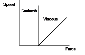
Frictional forces affect both the dynamic and steady-state response of the system. The force required to overcome friction is usually expressed as a function of velocity and the energy used is converted to heat and lost to the environment.
The forms of friction are usually classified as:
In many applications coulomb and viscous friction predominate.
It is convenient to plot the load characteristics in terms of speed and force (or torque) which will provide a means for matching them with those of the hydraulic system where flow is related to speed and pressure related to force.
2 Valve characteristics
Orifices are the principal control devices in fluid power systems. Usually they take the form of a circular hole or, as in the case of hydraulic control valves, an annular ring formed between a spool valve and the valve body.
2 Orifice flow
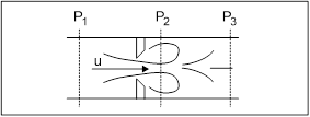
Figure 1 - Sharp edged orifice.
From elementary dynamic considerations, it can be shown for an incompressible fluid that the fluid velocity through the vena contracta, Figure 1 may be found using the following relationship:
where u = Fluid velocity m s-1
g = Gravimetric constant m s-2
h = Head across orifice m
P1 = Up stream pressure N m-2
P2 = Vena contracta pressure N m-2
P3 = Down stream pressure N m-2
r= Fluid density kg m-3 (870 for hydraulic oil)
3 Velocity
The local maximum velocity in an ideal case can be expressed in terms of the pressure drop. For example, if an orifice has a 100 bar differential pressure and the fluid density is 870 kg m-3, then:
![]()
4 Discharge Coefficient
A flow, Q, through an orifice can be related to the area and the velocity. Generally:
where Ao = orifice area m2
Equations (1) and (3) can be combined to obtain a relationship between the flow rate and the differential pressure across the orifice. The area at the vena contracta is reduced in relation to Ao, and a discharge coefficient Cd is included giving:
![]() (4)
(4)
For high flow rates indicated by a high Reynolds Number, the discharge coefficient for a sharp edged orifice has been shown to be 0.62. For other shapes, guiding the flow path more effectively, higher values can be obtained. For example, a Cd of 0.98 is possible for a nozzle.
The orifice equation (4) is obtained by making the following assumptions:
5 Flow Coefficients
In the practical case of a control orifice the conditions at the vena contracta are not easily measured. It is usual to relate the flow through the orifice to the pressure drop from inlet to outlet. In this case we can use a similar law with a flow coefficient Cq instead of the discharge coefficient.
Note that if the orifice area is very much less than the upstream area and the pressure P3 is the same as that at the vena contracta, then:
6 Variation in Flow Coefficient
The orifice flow coefficients change with the nature of the flow through the orifice (Reynolds Number Re effect). A convenient type of Reynolds Number, to use is often termed the flow number, [l].
For most sections:
wherel = Flow Number
Dh = Hydraulic diameter m
n= Kinematic viscosity m2 s-1
The relationship between the flow coefficient and the flow number can be seen in Figure 2
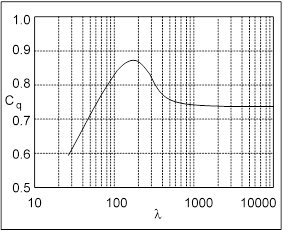
Figure 2 - Relationship between the flow coefficient and the flow number.
When the coefficient reaches a steady value at high l, then the flow equation can be considered a good representation of the actual situation. Where l is varying, the equation is not such an accurate description. Indeed at low flow numbers the flow in fact becomes directly proportional to the pressure drop across the orifice. At intermediate flows, the situation cannot be easily described mathematically.
7 Pressure Recovery Downstream of the Vena Contracta
Considering the expansion downstream of the vena contracta as a sudden enlargement shows the theoretical reason for the pressure recovery.
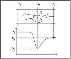
Figure 3 - Pressure characteristics through a sharp edge orifice.
By considering the momentum force at 3, assuming that the pressure at the vena contracta, P2 is constant across the pipe diameter:
The pressure P3 is determined by the resistance or load in the system down stream of the orifice. If this pressure is very low, it follows that the pressure at the vena contracta will be very low. In some cases it will be so low that air is released from the oil (saturation pressure). Below this at the vapour pressure air and vapour will be released into the fluid causing cavitation damage to occur. In addition to cavitation, the vapour bubbles will condense when the fluid enters a higher pressure region and the air will remain as bubbles. Whilst some of these will be released to the atmosphere in the reservoir, many will remain within the system. This may cause a spongy system operation and in extreme cases reduce the pump discharge.
Using the orifice equation the valve flow is given:
![]()
Thus the flow variation through a valve, for a given opening area, varies as the square root of ![]() , the magnitude of which will be limited by the supply pressure, Ps. In practice, the system designer is more concerned with the pressure difference, Pm, that is available across the actuator or motor and, consequently, it is more convenient to relate the flow to the actuator load pressure difference. The supply pressure, PS, is assumed to be constant.
, the magnitude of which will be limited by the supply pressure, Ps. In practice, the system designer is more concerned with the pressure difference, Pm, that is available across the actuator or motor and, consequently, it is more convenient to relate the flow to the actuator load pressure difference. The supply pressure, PS, is assumed to be constant.
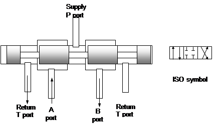
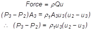
Figure 4 Spool Type Control Valve
For the spool type valve of Figure 4, movement of the spool in the direction shown will connect the B port to the outlet and the A port to the return line to the reservoir, or tank. This type of valve has three positions and is used as a directional control valve DCV. Various configurations are available for the centre position, which are discussed later. For partial openings of the valve there will be a restriction in the flow created by the lands of the valve as shown in Figure 5.
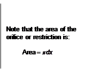
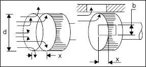
Figure 5 Orifice Restriction in Spool Valves
 In spool valves, there is a peripheral flow of fluid through the annulus formed by the valve land and the port as shown in Figure 5.
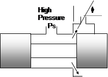
Figure 6 Spool valve
The flow from the high pressure inlet to the spool valve in Figure 6 creates a high velocity in the outlet metering annulus so that there is a resulting force on the spool tending to close the valve. This arises from the difference between the pressure force on the spool land on the left side, which is due to the inlet pressure, PS, and that on the right hand spool land, which is less because the pressure is reducing radially outwards due to the increasing fluid velocity. This pressure force is equal to the axial component of the momentum change so for a velocity U, the momentum force is given by:
![]()
The flow angle f depends on the valve opening and the clearance between the spool and the valve bore but it is often given the value of 690 attributed to the original work by Von Mises.
Four way valves can be used to control the velocity of actuators by introducing both meter-in and meter-out restrictions into the flow path as shown in Figure 7.
The valve position is fully variable and can be controlled by:
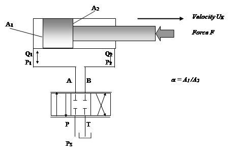
Figure 7 Four Way Valve Velocity Control
For proper design of the circuit and appropriate component selection it is necessary to analyse the system in order to determine the actuator pressures as a function of the actuator load force. In this system the pressure drop across each valve land needs to be considered as a function of the flow and the valve position or opening.
9 Analysis of the valve/actuator system
9.1 Actuator extending
Valve flow characteristics
For the parameters shown in Figure 6 the valve flows are given by:
![]()
![]()
where R1 = effective metering shape parameter (e.g. ![]() for annular ports).
for annular ports).
For zero pressure in the return line:
![]()
![]()
where R2 = effective metering area
 Also,
Also, ![]()
These equations give:
![]()
For a valve spool that has symmetrical metering, RS= 1
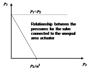
Figure 8 Valve Pressures during Extension
Equation 1 relates the pressures P1 and P2 for the valve connected to the unequal area actuator
as represented Figure 8. The flow from the annulus is lower than that to the piston because of its smaller area which results in a lower pressure drop in the valve.
Actuator force
![]()
![]() (2)
(2)
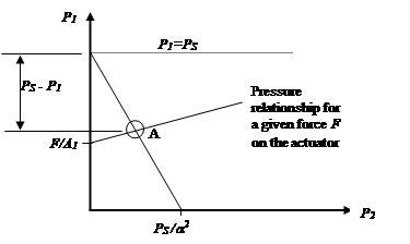
Figure 9 Interaction between the flow and the force characteristics during extension
Equation 2 relates the actuator pressures for a given actuator force with a positive force that acts in the opposing direction to the extending movement of the actuator. This relationship is shown on Figure 9 and the pressures for the valve controlling the actuator are determined by the intersection of the lines for the actuator and the valve at point A.
The values of these pressures can be obtained from equations 1 and 2 for the valve and actuator. The force acting on the actuator can be in either direction.
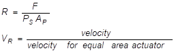
Using a force ratio defined by:
![]()
we get:
![]() (3)
(3)
and ![]() (4)
(4)
Variations of the force will change the position of the line on Figure 9 that represents the actuator and, hence, change the position of the point of intersection, A, that will change the pressure levels according to Equations 3 and 4.
For a value of R = 1, the force will be the maximum available and is the stall force for the system. For a given application the actuator area is chosen to provide the desired stall force at the chosen supply pressure. This will then determine the actuator pressures that are obtained for any other value of the force.
9.2 Actuator retracting
For retraction of the actuator the valve position is reversed, the annulus now being connected to the supply and the piston to the return line. Following the same method for a symmetrical valve (K1 = K2 )as for the actuator extension we get:
and ![]()
and as ![]()
Then ![]() (5)
(5)
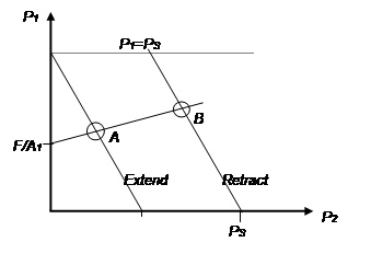
Figure 10 Actuator retracting
This relationship between P1 and P2 for the retracting actuator is shown in Figure 10 where point B is the operating condition for retraction of the actuator. It can be seen that when the valve is reversed there is a pressure change between points A and B.
The equations for the pressures for actuator retraction are:
![]() (5)
(5)
![]() (6)
(6)
The actuator velocity is determined from the flow equation for the valve using the appropriate values for the pressures P1 and P2. The selection of a valve having the necessary capacity is determined from the maximum required velocity condition.
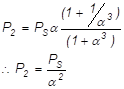
It should be noted that neither of the pressures can be less than zero so, for example, during extension, the maximum value of the force ratio, R, that is permissible in order to avoid cavitation of the flow to the piston is given by:
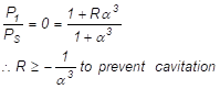
For which condition:
![]()
9.3 Valve sizing
The valve size needs to be selected such as to provide the flow required for the specified velocity and force conditions. In general, it is desirable to operate the system close to its condition of maximum efficiency, which can be obtained by considering the power transfer process.
For simplicity consider an equal area actuator for which the power transmitted to the load is given by;
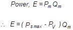
Here, PV is the valve pressure drop which, from the orifice equation, can be expressed as:
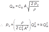
where A = the valve orifice area.
Hence:
For maximum power at the load:
and ![]() giving
giving ![]()
Based on this analysis an approximation is often applied from the maximum power condition to give the best combination of valve and actuator sizes for a given supply pressure such that the thrust at maximum power is equal to two-thirds the stall force.
The actuator size and the supply pressure can be selected to provide this stall thrust and the valve size is then determined on the basis of the maximum required value of ![]() .
.
Valves are rated by determining the flow at a total fixed pressure drop across both ports and for a given valve position. Thus the flow at any other pressure drop is given by:
![]()
Where QR = rated flow and DPR = rated pressure drop. DPR is sometimes given as the pressure drop through only one of the metering lands.
9.4 Valves with non-symmetrical metering
The use of valves in which the metering is non-symmetrical, normally by machining metering notches of different shapes, provides two major advantages over symmetrical valves which are:
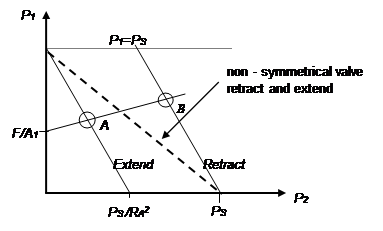
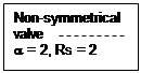
Figure 11 Non-symmetrical valve metering
The dotted line on Figure 11 shows the characteristics where the valve metering ratio, RS, has the same value as the actuator area ratio, a.
Figure 12 shows the output velocity U plotted against the force ratio R in comparison with the particular case of an equal area ratio actuator for which a =1. The equal area actuator has a symmetrical characteristic and is often used in servo systems for this reason. The dotted line shows the effect of asymmetrical metering where the valve-metering ratio is the same as the area ratio of the actuator.
![]()
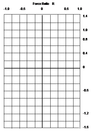
a = 2
a = 1
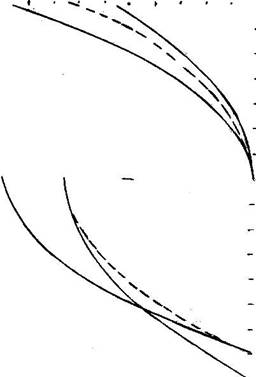
Figure 12 Load locus of velocity ratio against force ratio
This type of valve is used extensively for the operation of linear actuators in mobile systems but its major disadvantages are:
However, this type of control is simple, employs relative few moving parts and provides ease of control by the operator. An example of this type of system is that used for positioning the mobile crane jib the velocity of which responds quickly to the valve position selected by the crane operator. When the valve is put to the centre position its ports are blocked and the fluid between the valve and the actuator is trapped thus locking the actuator into its set position. Alternative valve control methods to reduce the power loss are discussed later.
A single pump can supply several valves where, in simple systems the pressure of a fixed displacement pump can be controlled by a relief valve. This system will increase the total power loss and bypass valves and/or variable displacement pumps with pressure compensation and load sensing are used to improve the overall efficiency. These methods are discussed in later sections.
This method of valve control can also be used to control the speed of hydraulic motors but, wherever possible, because of the continuous power loss in the valve it is preferable to connect the motor directly to the pump as a hydrostatic transmission.
The position of spool type valves can be controlled manually as shown in Figure 13 using a direct acting lever for its operation.
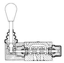
Figure 13 Manually Operated DCV
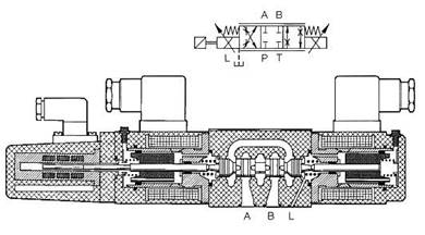
Figure 14 DC Solenoid Operated Proportional Valve
Valve position is often controlled using electrical solenoids for either AC or DC supplies. Proportional valves use a DC voltage input (usually ± 10V) to provide a continuously variable valve position, an example of this type of valve is shown in Figure 14.
10 Load Holding Valves
The radial clearance between the valve and its housing is carefully controlled in the manufacturing process to levels of around 2 micron. The leakage through this space, even at high pressures, is small but for applications where it is essential that the actuator remains in the selected position for long periods of time (e.g. crane jibs where any movement would be unacceptable) valves having metal-to-metal contact have to be used.
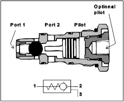
Figure 15 Pilot operated Check Valve
Check valves such as that in Figure 15 usually employ metal-to-metal contact but they are only open in one direction under the action of the flow into the valve. For their use in actuator circuits it is necessary that they are open in both directions as required by the DCV. This function can be obtained from a Pilot Operated Check Valve that uses a control pressure to open the valve against reverse flow
Figure 8 shows a typical pilot operated check valve (POCV) whereby a pilot pressure is applied onto the piston to force open the ball check valve to allow flow to pass from port 1 to port 2 when the check valve would normally be closed. The ratio of the piston and valve seat areas has to be chosen so that the available pilot pressure can provide sufficient force to open the valve against the pressure on port 1.
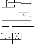
Figure 16 Actuator Circuit using a POCV
The use of a POCV is shown in Figure 16 where the external force on the actuator is acting in the extend direction. With the DCV in the centre position the check valve will be closed because the pilot is connected to the tank return line, which is at low pressure. Opening the DCV so as to extend the actuator the piston side pressure, now connected to the supply, will increase.
When this pressure reaches the level at which the check valve is opened against the pressure generated on the rod side of the actuator by the load force, the actuator will extend. The POCV acts as a restrictor and opens just sufficiently to allow the annulus flow to pass through at a pressure that just resists the force on the actuator.
Source: http://www.ivt.ntnu.no/ept/fag/tep4195/innhold/Forelesninger/hydraulikknotater%20fra%20Peter/Valvecontrol0406.doc
Web site to visit: http://www.ivt.ntnu.no
Author of the text: indicated on the source document of the above text
If you are the author of the text above and you not agree to share your knowledge for teaching, research, scholarship (for fair use as indicated in the United States copyrigh low) please send us an e-mail and we will remove your text quickly. Fair use is a limitation and exception to the exclusive right granted by copyright law to the author of a creative work. In United States copyright law, fair use is a doctrine that permits limited use of copyrighted material without acquiring permission from the rights holders. Examples of fair use include commentary, search engines, criticism, news reporting, research, teaching, library archiving and scholarship. It provides for the legal, unlicensed citation or incorporation of copyrighted material in another author's work under a four-factor balancing test. (source: http://en.wikipedia.org/wiki/Fair_use)
The information of medicine and health contained in the site are of a general nature and purpose which is purely informative and for this reason may not replace in any case, the council of a doctor or a qualified entity legally to the profession.
The texts are the property of their respective authors and we thank them for giving us the opportunity to share for free to students, teachers and users of the Web their texts will used only for illustrative educational and scientific purposes only.
All the information in our site are given for nonprofit educational purposes