VI. VISCOUS INTERNAL FLOW
To date, we have considered only problems where the viscous effects were either:
a. known: i.e. - known FD or hf
b. negligible: i.e. - inviscid flow
This chapter presents methodologies for predicting viscous effects and viscous flow losses for internal flows in pipes, ducts, and conduits.
Typically, the first step in determining viscous effects is to determine the flow regime at the specified condition.
The two possibilities are:
a. Laminar flow
b. Turbulent flow
The student should read Section 6.1 in the text, which presents an excellent discussion of the characteristics of laminar and turbulent flow regions.
For steady flow at a known flow rate, these regions exhibit the following:
Laminar flow: A local velocity constant with time, but which varies spatially due to viscous shear and geometry.
Turbulent flow: A local velocity which has a constant mean value but also has a statistically random fluctuating component due to turbulence in the flow.
Typical plots of velocity time histories for laminar flow, turbulent flow, and the region of transition between the two are shown below.
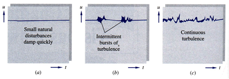
Fig. 6.1 (a) Laminar, (b)transition, and (c) turbulent flow velocity time histories.
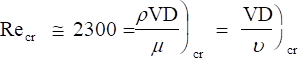
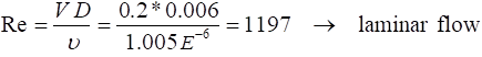
Principal parameter used to specify the type of flow regime is the
Reynolds number, 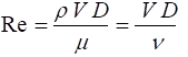
![]() - characteristic flow velocity
- characteristic flow velocity
D - characteristic flow dimension
m - dynamic viscosity
![]() - kinematic viscosity =
- kinematic viscosity = ![]()
We can now define the
Recr º critical or transition Reynolds number
Recr º Reynolds number below which the flow is laminar,
above which the flow is turbulent
While transition can occur over a range of Re, we will use the following for internal pipe or duct flow:
Internal Viscous Flow
A second classification concerns whether the flow has significant entrance region effects or is fully developed. The following figure indicates the characteristics of the entrance region for internal flows. Note that the slope of the streamwise pressure distribution is greater in the entrance region than in the fully developed region (due to frictional effects plus the acceleration of the core flow as the boundary layer develops).
Typical criteria for the length of the entrance region are given as follows:
Laminar: ![]()
Turbulent ![]()
where: Le = length of the entrance region
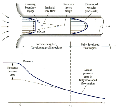
Note: Take care in neglecting entrance region effects.
In the entrance region, frictional pressure drop/length > the pressure drop/length for the fully developed region. Therefore, if the effects of the entrance region are neglected, the overall predicted pressure drop will be low. This can be significant in a system with short tube lengths, e.g. some heat exchangers.
Fully Developed Pipe Flow
The analysis for steady, incompressible, fully developed, laminar flow in a circular horizontal pipe yields the following equations:
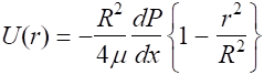
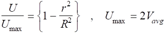
and
Q = A Vavg = p R2 Vavg
Key Points: Thus for laminar, fully developed pipe flow (not turbulent):
a. The velocity profile is parabolic.
b. The maximum local velocity is at the centerline (r = 0).
c. The average velocity is one-half the centerline velocity.
d. The local velocity at any radius varies only with radius, not on the streamwise (x) location (due to the flow being fully developed).
Note: All subsequent equations will use the symbol V (no subscript) to represent the average flow velocity in the flow cross section.
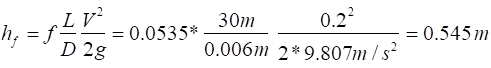
Darcy Friction Factor:
We can now define the Darcy friction factor f as:
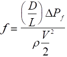 |
where DPf = the pressure drop due to friction only. |
Therefore, we obtain
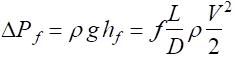
and the friction head loss hf is given as
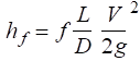
Note: The definitions for f and hf are valid for either laminar or turbulent flow. However, you must evaluate f for the correct flow regime, laminar or turbulent.
Key Point: It is common in industry to define and use a “fanning” friction factor ff in viscous pipe flow analyses. The fanning friction factor differs from the Darcy friction factor by a factor of 4.
Thus, care should be taken when using unfamiliar equations or data since use of ff in equations that were developed for the Darcy friction factor will result in significant errors (a factor of 4).
Your employer will not be happy if you order a 10 hp motor for a 2.5 hp application. The equation suitable for use with ff is
fanning friction factor only: 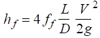
Laminar flow:
Application of the results for the laminar flow velocity profile to the definition of the Darcy friction factor yields the following expression:
 laminar flow only (Re < 2300)
Thus, with the value of the Reynolds number, the friction factor for laminar flow is easily determined.
Turbulent flow:
A similar analysis is not readily available for turbulent flow. However, the Colebrook equation, shown below, provides an excellent representation for the variation of the Darcy friction factor in the turbulent flow regime. Note that the equation depends on both the pipe Reynolds number and the roughness ratio, is transcendental, and cannot be expressed explicitly for f .
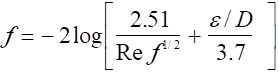 turbulent flow only (Re > 2300)
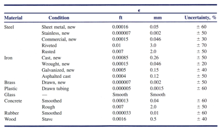
where e = nominal roughness of pipe or duct being used. (Table 6.1, text)
(Note: Take care with units for e; e /D must be non-dimensional)
A good approximate equation for the turbulent region of the Moody chart is given by Haaland’s equation:
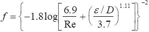
Note again the roughness ratio e/D must be non-dimensional in both equations.
Graphically, the results for both laminar and turbulent flow pipe friction are represented by the Moody chart as shown below.
Typical roughness values are shown in the following table:
Table 6.1 Average roughness values of commercial pipe
Haaland’s equation is valid for turbulent flow (Re > 2300) and is easily set up on a computer, spreadsheet, etc.
Key fluid system design considerations for laminar and turbulent flow
a. Most internal flow problems of engineering significance are turbulent, not laminar. Typically, a very low flow rate is required for internal pipe flow to be laminar. If you open your kitchen faucet and the outlet flow stream is larger than a kitchen match, the flow is probably turbulent. Thus, check your work carefully if your analysis indicates laminar flow.
b. The following can be easily shown:
Laminar flow: ![]()
![]()
![]()
Turbulent flow: ![]()
![]()
The subscript ‘f’ on each of these terms indicates that these represent the effects due to friction only and are not the total pressure drop or power requirements.
Thus, both pressure drop and pump power are very dependent on flow rate and pipe/conduit diameter. Small changes in diameter and/or flow rate can significantly change circuit pressure drop and power requirements.
Example ( Laminar flow): |
|
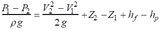
Water Properties: Energy Equation (neglecting a)
r = 998 kg/m3 rg = 9790 N/m3 n = 1.005 E-6 m2/s |
|
which for steady-flow in a constant diameter pipe with P2 = 0 gage becomes, |
|
![]()
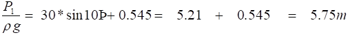
gravity friction total head
head head loss
P1 = 9790 N/m3*5.75 m = 56.34 kN/m3 (kPa) ~ 8.2 psig ans.
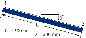
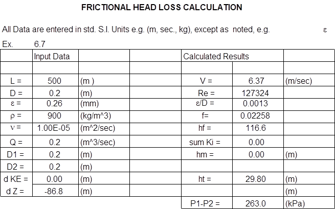
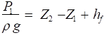
Example (turbulent flow): |
|
The energy equation for a = 1 can be written as follows where ht = total head loss. |
|
which reduces to |
|
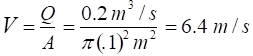 Table 6.1, cast iron, e = 0.26 mm
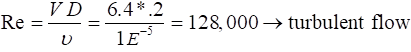 ,
, 
Since flow is turbulent, use Haaland’s equation to determine friction factor (check your work using the Moody chart).
 ,
, 
![]()
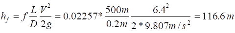 ans.
ans.
ht = Z2 – Z1 + hf = - 500 sin 0 + 116.6 = - 86.8 + 116.6 = 29.8 m ans.
Note that for this problem, there is a negative gravity head loss (i.e. a head increase) and a positive frictional head loss resulting in the net head loss of 29.8 m.
![]() ans.
ans.
![]() ans.
ans.
Note that this is not necessarily the power required to drive a pump, as the pump efficiency will typically be less than 100%.
These problems are easily set up for solution in a spreadsheet as shown below. Make sure that the calculation for friction factor includes a test for laminar or turbulent flow (i.e. Re > or < 2300) with the analysis then using the correct equation for friction factor, f.
Always verify any computer solution with problems having a known solution.
Solution Summary:
To solve basic pipe flow frictional head loss problem, use the following procedure:
1. Use known flow rate to determine Reynolds number.
2. Identify whether flow is laminar or turbulent.
3. Use correct expression to determine friction factor (with e/D if necessary).
4. Use definition of hf to determine friction head loss.
5. Use general energy equation to determine total pressure drop.
Unknown Flow Rate and Diameter Problems
Problems involving unknown flow rate and diameter in general require iterative/ trial & error solutions due to the complex dependence of Re, friction factor, and head loss on velocity and pipe size.
Unknown Flow Rate:
For the special case of known friction loss, hf , a closed form solution can be obtained for the problem of unknown Q.
The solution proceeds as follows:
Given: Known values for D, L, hf, r, and m , calculate V or Q.
(Note: It is the friction head loss, hf, not the total head loss, ht, used in the solution.
Define solution parameter:
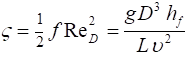
Note that this solution does not contain velocity and the parameter z can be calculated from known values for D, L, hf, r, and m. The Reynolds number and subsequently the velocity can be determined from z and the following equations:
Turbulent: 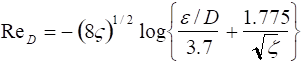
Laminar: ![]()
and laminar to turbulent transition can be assumed to occur approximately at
z = 73,600 (check Re at end of calculation to confirm).
Note that this procedure is not valid (except perhaps for initial estimates) for problems involving significant minor losses where the head loss due only to pipe friction is not known.
For these problems a trial and error solution using a computer is best. For example, using the previous spreadsheet, assume values for Q until the correct ht is obtained.
Example 6.9
Oil, with r = 950 kg/m3 and n = 2 E-5 m2/s, flows through 100 m of a 30 cm diameter pipe. The pipe is known to have a head loss of 8 m and a roughness ratio e/D = 0.0002. Determine the flow rate and oil velocity possible for these conditions.
Without any information to the contrary, we will neglect minor losses and KE head changes. With these assumptions, we can write:
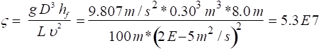 > 73,600; turbulent
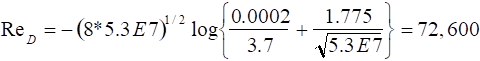 checks, turbulent
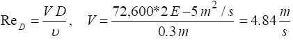 ans.
ans.
![]() ans.
ans.
This is the maximum flow rate and oil velocity that could be obtained through the given pipe and given conditions (hf = 8 m).
Again, this problem could have also been solved using a computer based trial and error procedure in which a value is assumed for the fluid flow rate until a flow rate is found which results in the specified head loss.
Note also that with a more general computer based procedure, the problem being solved can include the effects of minor losses, KE, and PE changes with no additional difficulty.
Unknown Pipe Diameter:
A similar difficulty arises for problems involving unknown pipe difficulty, except a closed form, analytical solution is not generally available. Again, a trial and error solution is appropriate for use to obtain the solution and the problem can again include losses due to KE, PE, and piping components with no additional difficulty. This procedure is shown in the following example using the previous spreadsheet based solution.
Ex. 6.11 A fluid with the indicated properties is known to flow through a 100 m long pipe with e = .06 mm and a flow rate of 0.342 m3/s and a frictional head loss, hf = 8 m. What diameter pipe is required to provide these conditions?
Again, assume values of D until the value of hf = 8 m is obtained in the solution.

Source: http://www.eng.auburn.edu/~tplacek/courses/2610/samba/CHEN2610FacultyCh6a.doc
Web site to visit: http://www.eng.auburn.edu
Author of the text: indicated on the source document of the above text
If you are the author of the text above and you not agree to share your knowledge for teaching, research, scholarship (for fair use as indicated in the United States copyrigh low) please send us an e-mail and we will remove your text quickly. Fair use is a limitation and exception to the exclusive right granted by copyright law to the author of a creative work. In United States copyright law, fair use is a doctrine that permits limited use of copyrighted material without acquiring permission from the rights holders. Examples of fair use include commentary, search engines, criticism, news reporting, research, teaching, library archiving and scholarship. It provides for the legal, unlicensed citation or incorporation of copyrighted material in another author's work under a four-factor balancing test. (source: http://en.wikipedia.org/wiki/Fair_use)
The information of medicine and health contained in the site are of a general nature and purpose which is purely informative and for this reason may not replace in any case, the council of a doctor or a qualified entity legally to the profession.
The texts are the property of their respective authors and we thank them for giving us the opportunity to share for free to students, teachers and users of the Web their texts will used only for illustrative educational and scientific purposes only.
All the information in our site are given for nonprofit educational purposes
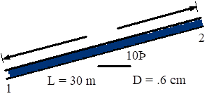
 = L sin 10o + hf