1.       Objectives

1.1       Analyse fixed and variable cost elements from total cost data using high/low and regression methods.
1.2       Explain the use of forecasting techniques, including time series, simple average growth models and estimates based on judgement and experience. Predict a future value from provided time series analysis data using both additive and proportional data.
1.3       Estimate the learning effect and apply the learning curve to a budgetary problem, including calculations on steady states.
1.4       Discuss the reservations with the learning curve.
1.5       Explain the benefits and dangers inherent in using spreadsheets in budgeting.

2.       Analysing Fixed and Variable Costs

2.1       Two important quantitative methods the management accountant can use to analyse fixed and variable cost elements from total cost data are the high-low and regression methods.

2.2       The high-low method

2.2.1    A method of analysing a semi-variable cost into its fixed and variable elements based on an analysis of historical information about costs at different activity levels.

2.2.2

The steps of high-low method

Step 1:    Select the highest and lowest activity levels, and their costs. (Note: do not take the highest and lowest cost). Step 2:    Find the variable cost per unit. Cost at high level of activity – Cost at low level of activity High level activity – Low level activity Step 3:    Find the fixed cost, using either the high or low activity level. Fixed cost = Total cost at activity level – Total variable cost

2.2.3    The high-low method has the enormous advantage of simplicity. It is easy to understand and easy to use.
2.2.4    The limitations of the high-low method are:
(a)        The method ignores all cost information apart from at the highest and lowest volumes of activity.
(b)        Inaccurate cost estimates may be produced as a result of the assumption of a constant relationship between costs and volume of activity.
(c)        Estimates are based on historical information and conditions may have changed.

 

 

2.2.5

Example 1

Cost data for the six months to 31 December 2011 is as follows: Month Units Inspection costs     $ July 340 2,240 August 300 2,160 September 380 2,320 October 420 2,400 November 400 2,360 December 360 2,280 The variable element of a cost item is estimated calculating the unit cost between high and low volumes during a period.   Units Inspection costs     $ Highest level 420 2,400 Lowest level 300 2,160 Difference 120 240 Variable cost per unit = $240 ÷ 120 = $2 per unit Fixed inspection costs are, therefore: $2,400 – (420 units × $2) = $1,560 per month Or $2,160 – (300 units × $2) = $1,560 per month i.e. the relationship is of the form y = $1,560 + $2x

2.3       Linear regression analysis

2.3.1    Regression involves using historical data to find the line of best fit between two variables (one dependent on the other), and use this to predict future values.

2.3.2

Linear relationships

(a)       A linear relationship can be expressed in the form of an equation which has the general form: y = a + bx Where y is the dependent variable, depending for its value on the value of x, e.g. the total costs x is the independent variable, e.g. units a is a constant, e.g. fixed cost b is a constant, e.g. variable cost (b)       To find the line of best fit we need to calculate a and b using the historical data for x and y. The formulae for these are: Where n is the number of pair of data for x and y.

 

2.3.4    The strength of the linear relationship between the two variables (and hence the usefulness of the regression line equation) can be assessed by calculating the correlation coefficient (“r”) and the coefficient of determination (“r2”), where

2.3.5    If the degree of association between the two variables is very close, it will be almost possible to plot the observations on a straight line, and r and r2 will be very near to 1. In this situation a high correlation between costs and activity exists.
2.3.6    At the other extreme, costs may be so randomly distributed that there is little or no correlation between costs and the activity base selected. The r2 calculation will be near to zero.

2.3.7	Example 3
	Using the date from Example 2 above: Thus 95.7% of the observed variation is sales can be explained as being due to changes in the advertising spending. This would give strong assurances that the forecasts made using the regression equation are valid.

3.       Time Series Analysis

3.1       A time series is a series of figures relating to the changing value of a variable over time. The data often conforms to a certain pattern over time. This pattern can be extrapolated into the future and hence forecasts are possible. Time periods may be any measure of time including days, weeks, months and quarters.

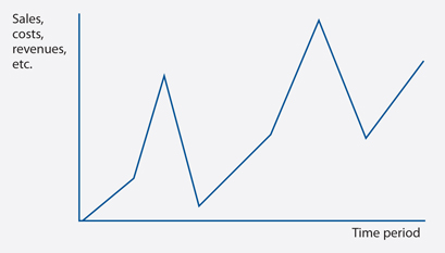
3.2       The four components of a time series are:
(a)        The trend – this describes the long-term general movement of the data.
(b)        Seasonal variations – a regular variation around the trend over a fixed time period, usually one year.
(c)        Cyclical variations – are commonly associated with economic cycle of booms and slumps.
(d)        Residual variations – irregular, random fluctuations in the data usually caused by factors specific to the time series. They are unpredictable.
3.3       In practice a time series could incorporate all of the four features we have been looking at and, to make reasonably accurate forecasts, the four features often have to be isolated. We can begin the process of isolating each feature by summarizing the components of a time series as follows.

The actual time series, Y = T + S + C + R

Y = the actual time series
T = the trend series
S = the seasonal component
C = the cyclical component
R = the residual or random component
3.4       Though you should be aware of the cyclical component, it is unlikely that you will be expected to carry out any calculation connected with isolating it. The mathematical models which we will use therefore excludes any reference to C.

3.5       Finding the seasonal variations – additive model

3.5.1    The additive model for time series analysis is Y = T + S + R. We can therefore write Y – T = S + R.
3.5.2    In other words, if we deduct the trend series from the actual series, we will be left with the seasonal and random components of the time series. If we assume that the random component is relatively small, and hence negligible, the seasonal component can be found as S = Y – T, the de-trend series.
3.5.3    This model assumes that the components of the series are independent of each other, so that increasing trend does not affect the seasonal variations and make them increase as well.

 

            Finding the seasonal variations – proportional (multiplicative) model

3.6.1    The proportional model summarises a time series as Y = T × S × R.
3.6.2    The trend component will be the same whichever model is used but the values of the seasonal and random components will vary according to the model being applied.

3.6.3

Exercise 2

A company has found that the trend in the quarterly sales of its furniture is well described by the regression equation Y = 150 + 10X Where Y equals quarterly sales X = 1 represents the first quarter of 2012 X = 2 represents the second quarter of 2012 X = 5 represents the first quarter of 2013, etc. It has also been found that, based on a multiplicative model, i.e. Sales = Trend × Seasonal × Random The mean seasonal quarterly index for its furniture sales is as follows: Quarter 1 2 3 4 Seasonal index 80 110 140 70 Required: (a)       Explain the meaning of this regression equation, and set of seasonal index numbers. (b)       Using the regression equation, estimate the trend values in the company’s furniture sales for each quarter of 2017. (c)       Using the seasonal index, prepare sales forecasts for the company’s quarterly furniture sales in 2017. (d)       State the factors might cause your sales forecasts to be in error.

 

Solution:

3.7       Time series analysis and forecasting

3.7.1    Forecasts of future values should be made as follows.
(a)        Find a trend line using moving averages or using linear regression analysis.
(b)       Use the trend line to forecast future trend line values.
(c)        Adjust these values by the average seasonal variation applicable to the future period, to determine the forecast for that period. With the additive model, add (or subtract for negative variations) the variation. With the multiplicative model, multiply the trend value by the variation proportion.

3.8       Forecasting problems

3.8.1    All forecasts are subject to error, but the likely errors vary from case to case.
(a)        The further into the future the forecast is for, the more unreliable it is likely to be
(b)       The less data available on which to base the forecast, the less reliable the forecast
(c)        The historic pattern of trend and seasonal variations may not continue in the future
(d)       Random variations may upset the pattern of trend and seasonal variation
(e)        Extrapolation of the trend line is done by judgment and can introduce errors
3.8.2    There are a number of changes that also may make it difficult to forecast future events.

Type of change	Examples
Political and economic changes	Changes in interest rates, exchange rates or inflation can mean that future sales and costs are difficult to forecast.
Environmental changes	The opening of high-speed rail links might have a considerable impact on some companies' markets.
Technological changes	These may mean that the past is not a reliable indication of likely future events. For example new faster machinery may make it difficult to use current output levels as the basis for forecasting future production output.
Technological advances	Advanced manufacturing technology is changing the cost structure of many firms. Direct labour costs are reducing in significance and fixed manufacturing costs are increasing. This causes forecasting difficulties because of the resulting changes in cost behaviour patterns, breakeven points and so on.
Social changes	Alterations in taste, fashion and the social acceptability of products can cause forecasting difficulties.

4.      Learning Curves

4.1       As workers become more familiar with the production of a new product, average time (and average cost) per unit will decline.
4.2       Learning curve theory applies to situations where the work force as a whole improves in efficiency with experience. The learning effect describes the speeding up of a job with repeated performance.
4.3       Where does learning curve theory apply?
(a)        Highly labour intensive production.
(b)        Brand new or relatively short-lived product, the learning process does not continue indefinitely.
(c)        Complex and made in small quantities for special orders.
4.4       There are three approaches to learning curve problems
(a)        The tabular approach
(b)        The graphical approach
(c)        The algebraic approach

4.5       Method 1 – The tabular approach: cumulative average time and the learning rate

4.5.1    The tabular approach is only effective in scenarios where output is doubling.

4.5.2

Example 4

The first unit of output of a new product requires 100 hours. An 80% learning curve applies. The production times would be as follows. No. of units produced Cumulative average time required per unit Total time required Incremental time for additional units 1   100.0 (× 1) 100.0     2* (80%) 80.0 (× 2) 160.0 60.0 (1 extra unit) 4* (80%) 64.0 (× 4) 256.0 96.0 (2 extra unit) 8* (80%) 51.2 (× 8) 409.6 153.6 (4 extra unit) * Output is being doubled each time.

4.6       Method 2 – The graphical approach

4.6.1    The learning effect from the above example can also be shown on a graph, as a learning curve either for unit times or cumulative total times or costs.

4.6.2    Whilst this approach is useful in scenarios where output is not doubling, in reality it is not as accurate as methods 1 and 3.

4.7       Method 3 – The algebraic approach

4.7.1

The algebraic approach

The formula for the learning curve is Y = axb, where b, the learning coefficient or learning index, is defined as (log of the learning rate/log 2). The learning curve formula can be used to solve all learning curve scenarios. Where:  Y is the cumulative average time per unit to produce x units x is the cumulative number of units a is the time taken for the first unit of output b is the index of learning [log (learning rate) / log 2]

 

4.7.2

Example 5

Suppose, for example, that an 80% learning curve applies to production of item ABC. To date (the end of June) 230 units of ABC have been produced. Budgeted production for July is 55 units. The cost of the very first unit of ABC, in January, was $120. Required: Calculate the budgeted total labour cost for July. Solution: To solve this problem, we need to calculate three things. (a)     The cumulative total labour cost so far to produce 230 units of ABC. (b)    The cumulative total labour cost to produce 285 units of ABC, that is adding on the extra 55 units for July. (c)     The extra cost of production of 55 units of ABC in July, as the difference between (b) and (a). Calculation (a) y = axb and we know that for 230 cumulative units, a = $120 (cost of first unit), x = 230 (cumulative units) and b = –0.322 (80% learning curve) and so y = 120 × (230–0.322) = $20.83. So when x = 230 units, the cumulative average cost per unit is $20.83. Calculation (b) Now we do the same sort of calculation for x = 285. If x = 285, y = 120 × (285–0.322) = $19.44 So when X = 285 units, the cumulative average cost per unit is $19.44. Calculation (c) Cumulative units Average cost per unit Total cost   $ $ 230 20.83 4,790.90 285 19.44 5,540.40 Incremental cost for 55 units   749.50 Average cost per unit, between 230 and 285 units = 749.50 / 55 = $13.63 per unit approx.

The practical application of learning curve theory

4.8.1    What costs are affected by the learning curve?
(a)        Direct labour time and costs
(b)       Variable overhead costs, if they vary with direct labour hours worked.
(c)        Materials costs are usually unaffected by learning among the workforce, although it is conceivable that materials handling might improve, and so wastage costs be reduced.
(d)       Fixed overhead expenditure should be unaffected by the learning curve (although in an organisation that uses absorption costing, if fewer hours are worked in producing a unit of output, and the factory operates at full capacity, the fixed overheads recovered or absorbed per unit in the cost of the output will decline as more and more units are made).

4.9       The relevance of learning curve effects in management accounting

4.9.1    Learning curve can be used to:
(a)        Calculate the marginal (incremental) cost of making extra units of a product.
(b)        Quote selling prices for a contract, where prices are calculated at cost plus a percentage mark-up for profit. An awareness of the learning curve can make all the difference between winning contracts and losing them, or between making profits and selling at a loss-making price.
(c)        Prepare realistic production budgets and more efficient production schedules.
(d)        Prepare realistic standard costs for cost control purposes.

4.10     Limitations of learning curve theory

4.10.1  Limitations:
(a)        The learning curve phenomenon is not always present.
(b)        It assumes stable conditions at work which will enable learning to take place. This is not always practicable, for example because of labour turnover.
(c)        It must also assume a certain degree of motivation amongst employees.
(d)        Breaks between repeating production of an item must not be too long, or workers will 'forget' and the learning process will have to begin all over again.
(e)        It might be difficult to obtain accurate data to decide what the learning curve is.
(f)        Workers might not agree to a gradual reduction in production times per unit.
(g)        Production techniques might change, or product design alterations might be made, so that it takes a long time for a 'standard' production method to emerge, to which a learning effect will apply.

5.      Using Spreadsheets in Budgeting

5.1       Advantages of spreadsheets
(a)        The great value of spreadsheets derives from their simple format of rows, columns and worksheets of data.
(b)        The ability of the data users to have direct access themselves to their spreadsheet model via their own PC.
(c)        It is easy to have instant access to the model whenever it is needed, in just the time it takes to load the model into the PC.
(d)        It can help to handle complex calculation and so it can save time.
5.2       Disadvantages of spreadsheets
(a)        A minor error in the design of a model at any point can affect the validity of data throughout the spreadsheet. Such errors can be very difficult to trace.
(b)        Even if it is properly designed in the first place, it is very easy to corrupt a model by accidentally changing a cell or inputting data in the wrong place.
(c)        It is possible to become over-dependent on them, so that simple one-off tasks that can be done in seconds with a pen and paper are done on a spreadsheet instead.
(d)        The possibility for experimentation with data is so great that it is possible to lose sight of the original intention of the spreadsheet.
(e)        Spreadsheets cannot take account of qualitative factors since they are invariably difficult to quantify. Decisions should not be made on the basis of quantitative information alone.

Examination Style Questions

Question 1 – Learning curve
BFG Limited is investigating the financial viability of a new product the S-pro. The S-pro is a short-life product for which a market has been identified at an agreed design specification. The product will only have a life of 12 months.

The following estimated information is available in respect of S-pro:

1.         Sales should be 120,000 in the year in batches of 100 units. An average selling price of $1,050 per batch of 100 units is expected. All sales are for cash.
2.         An 80% learning curve will apply for the first 700 batches after which a steady state production time will apply, with the labour time per batch after the first 700 batches being equal to the time for the 700th batch. The cost of the first batch was measured at $2,500. This was for 500 hours at $5 per hour.
3.         Variable overhead is estimated at $2 per labour hour.
4.         Direct material will be $500 per batch of S-pro for the first 200 batches produced. The second 200 batches will cost 90% of the cost per batch of the first 200 batches. All batches from then on will cost 90% of the batch cost for each of the second 200 batches. All purchases are made for cash.
5.         S-pro will require additional space to be rented. These directly attributable fixed costs will be $15,000 per month.

A target net cash flow of $130,000 is required in order for this project to be acceptable.

Note: The learning curve formula is given on the formulae sheet. At the learning rate of 0.8 (80%), the learning factor (b) is equal to -0.3219.

Required:

(a)        Prepare detailed calculations to show whether product S-pro will provide the target net cash flow.                                                                                                              (12 marks)
(b)        Calculate what length of time then second batch will take if the actual rate of learning is:
(i)         80%;
(ii)        90%.
Explain which rate shows the faster learning.                                        (5 marks)
(c)        Suggest specific actions that BFG could take to improve the net cash flow calculated above.      (8 marks)
(25 marks)
(ACCA F5 Performance Management Pilot Paper Q3)

Question 2 – Learning curve
Henry Company (HC) provides skilled labour to the building trade. They have recently been asked by a builder to bid for a kitchen fitting contract for a new development of 600 identical apartments. HC has not worked for this builder before. Cost information for the new contract is as follows:

Labour for the contract is available. HC expects that the first kitchen will take 24 man-hours to fit but thereafter the time taken will be subject to a 95% learning rate. After 200 kitchens are fitted the learning rate will stop and the time taken for the 200th kitchen will be the time taken for all the remaining kitchens. Labour costs $15 per hour.

Overheads are absorbed on a labour hour basis. HC has collected overhead information for the last four months and this is shown below:

	Hours worked	Overhead cost ($)
Month 1	9,300	115,000
Month 2	9,200	113,600
Month 3	9,400	116,000
Month 4	9,600	116,800

HC normally works around 120,000 labour hours in a year.

HC uses the high low method to analyse overheads.

The learning curve equation is y = axb, where b =

Required:

(a)        Describe FIVE factors, other than the cost of labour and overheads mentioned above, that HC should take into consideration in calculating its bid.                                       (10 marks)
(b)        Calculate the total cost including all overheads for HC that it can use as a basis of the bid for the new apartment contract.                                                                               (13 marks)
(c)        If the second kitchen alone is expected to take 21·6 man-hours to fit demonstrate how the learning rate of 95% has been calculated.                                                                   (2 marks)
(25 marks)
(ACCA F5 Performance Management December 2008 Q3)

Question 3 – Target costing and learning curve
Big Cheese Chairs (BCC) manufactures and sells executive leather chairs. They are considering a new design of massaging chair to launch into the competitive market in which they operate.

They have carried out an investigation in the market and using a target costing system have targeted a competitive selling price of $120 for the chair. BCC wants a margin on selling price of 20% (ignoring any overheads).

The frame and massage mechanism will be bought in for $51 per chair and BCC will upholster it in leather and assemble it ready for despatch.

Leather costs $10 per metre and two metres are needed for a complete chair although 20% of all leather is wasted in the upholstery process.

The upholstery and assembly process will be subject to a learning effect as the workers get used to the new design. BCC estimates that the first chair will take two hours to prepare but this will be subject to a learning rate (LR) of 95%. The learning improvement will stop once 128 chairs have been made and the time for the 128th chair will be the time for all subsequent chairs. The cost of labour is $15 per hour.

The learning formula is shown on the formula sheet and at the 95% learning rate the value of b is –0·074000581.

Required:

(a)     Calculate the average cost for the first 128 chairs made and identify any cost gap that may be present at that stage.                                                                                                  (8 marks)
(b)     Assuming that a cost gap for the chair exists suggest four ways in which it could be closed.          (6 marks)

The production manager denies any claims that a cost gap exists and has stated that the cost of the 128th chair will be low enough to yield the required margin.

(c)     Calculate the cost of the 128th chair made and state whether the target cost is being achieved on the 128th chair.                                                                                                         (6 marks)
(Total 20 marks)
(ACCA F5 Performance Management December 2009 Q2)

Question 4 – Demand function, learning curve and pricing strategies
Heat Co specialises in the production of a range of air conditioning appliances for industrial premises. It is about to launch a new product, the ‘Energy Buster’, a unique air conditioning unit which is capable of providing unprecedented levels of air conditioning using a minimal amount of electricity. The technology used in the Energy Buster is unique so Heat Co has patented it so that no competitors can enter the market for two years. The company’s development costs have been high and it is expected that the product will only have a five-year life cycle.

Heat Co is now trying to ascertain the best pricing policy that they should adopt for the Energy Buster’s launch onto the market. Demand is very responsive to price changes and research has established that, for every $15 increase in price, demand would be expected to fall by 1,000 units. If the company set the price at $735, only 1,000 units would be demanded.

The costs of producing each air conditioning unit are as follows:

Note
The first air conditioning unit took 1·5 hours to make and labour cost $8 per hour. A 95% learning curve exists, in relation to production of the unit, although the learning curve is expected to finish after making 100 units. Heat Co’s management have said that any pricing decisions about the Energy Buster should be based on the time it takes to make the 100th unit of the product. You have been told that the learning co-efficient, b = –0·0740005.

All other costs are expected to remain the same up to the maximum demand levels.

Required:

(a)        (i)        Establish the demand function (equation) for air conditioning units;
(3 marks)
(ii)        Calculate the marginal cost for each air conditioning unit after adjusting the labour cost as required by the note above;                                                        (6 marks)
(iii)       Equate marginal cost and marginal revenue in order to calculate the optimum price and quantity.                                                                                                    (3 marks)
(b)        Explain what is meant by a ‘penetration pricing’ strategy and a ‘market skimming’ strategy and discuss whether either strategy might be suitable for Heat Co when launching the Energy Buster.           (8 marks)
(20 marks)
(ACCA F5 Performance Management June 2011 Q2)

Question 5 – Life cycle costing and learning curve
Fit Co specialises in the manufacture of a small range of hi-tech products for the fitness market. They are currently considering the development of a new type of fitness monitor, which would be the first of its kind in the market. It would take one year to develop, with sales then commencing at the beginning of the second year. The product is expected to have a life cycle of two years, before it is replaced with a technologically superior product. The following cost estimates have been made.

Note: You should ignore the time value of money.

Required:

(a)        Calculate the life cycle cost per unit.                                                     (6 marks)
(b)        After preparing the cost estimates above, the company realises that it has not taken into account the effect of the learning curve on the production process. The variable manufacturing cost per unit above, of $40 in year 2 and $42 in year 3, includes a cost for 0·5 hours of labour. The remainder of the variable manufacturing cost is not driven by labour hours. The year 2 cost per hour for labour is $24 and the year 3 cost is $26 per hour. Subsequently, it has now been estimated that, although the first unit is expected to take 0·5 hours, a learning curve of 95% is expected to occur until the 100th unit has been completed.

Calculate the revised life cycle cost per unit, taking into account the effect of the learning curve.
Note: the value of the learning co-efficient, b, is –0·0740005.           (10 marks)
(c)        Discuss the benefits of life cycle costing.                                              (4 marks)
(20 marks)
(ACCA F5 Performance Management December 2011 Q4)

 

4.7.3

Example 6

A company needs to calculate a new standard cost for one of its products. When the product was introduced, the standard variable cost of the first unit was as follows.     Costs per unit     $ Direct material 10kg @ $3 per kg 30 Direct labour 10 hours @ $9 per hour 90 Variable overhead 10 hours @ $5 per hour 50 Total   170 During the following year, a 90% learning curve was observed. The cumulative production at the end of the third quarter was 50 units and the budgeted production for the fourth quarter is 10 units. Required: (a)       What is the standard cost per unit for the fourth quarter assuming that the 90% learning curve still applies? (b)       What is the standard cost per unit for the fourth quarter assuming the learning curve had reached a steady state i.e. peak efficiency was reached after the 50th unit was produced? Solution: (a) y = axb and for 60 cumulative units a = 10 hours (time for first unit), x = 60 (cumulative units) and b = –0.152 (90% learning curve) and so y = 10 × (60-0.152) = 5.37 hours. For 50 cumulative units y = 10 x (50-0.152) = 5.52 hours. Cumulative units Average time per unit Total time 50 5.52 276.0 60 5.37 322.2 Incremental time for 10 units   46.2 The standard time per unit is therefore 46.2/10 = 4.62 hours The standard cost per unit is:     Costs per unit     $ Direct material 10kg @ $3 per kg 30.00 Direct labour 4.62 hours @ $9 per hour 41.58 Variable overhead 4.62 hours @ $5 per hour 23.10 Total   94.68 (b) A steady state is reached after the 50th unit so we need the time taken to produce the 50th unit. For 49 cumulative units a = 10 hours (time for first unit), x = 49 (cumulative units) and b = -0.152 (90% learning curve) and so y = 10 x (49-0.152) = 5.535 hours. Cumulative units Average time per unit Total time 49 5.535 271.2 50 5.520 276.0 Incremental time for 50th units   4.8 The standard cost per unit is:     Costs per unit     $ Direct material 10kg @ $3 per kg 30.00 Direct labour 4.8 hours @ $9 per hour 43.20 Variable overhead 4.8 hours @ $5 per hour 24.00 Total   97.20

3.5.4

Exercise 1

The Western is a local government organisation responsible for waste collection from domestic households. The new management accountant of The Western has decided to introduce some new forecasting techniques to improve the accuracy of the budgeting. The next budget to be produced is for the year ended 31 December 2010. Waste is collected by the tonne (T). The number of tonnes collected each year has been rising and by using time series analysis the new management accountant has produced the following relationship between the tonnes collected (T) and the time period in question Q (where Q is a quarter number. So Q = 1 represents quarter 1 in 2009 and Q = 2 represents quarter 2 in 2009 and so on) T = 2,000 + 25Q Each quarter is subject to some seasonal variation with more waste being collected in the middle quarters of each year. The adjustments required to the underlying trend prediction are: Quarter Tonnes 1 -200 2 +250 3 +150 4 -100 Once T is predicted the new management accountant hopes to use the values to predict the variable operating costs and fixed operating costs that The Western will be subjected to in 2010. To this end he has provided the following operating cost data for 2009. Volume of waste Total operating cost in 2009 (fixed + variable) Tonnes $000s 2,100 950 2,500 1,010 2,400 1,010 2,300 990 Inflation on the operating cost is expected to be 5% between 2009 and 2010. The regression formula is shown on the formula sheet. Required: (a)       Calculate the tones of waste to be expected on the calendar year 2010. (4 marks) (b)       Calculate the variable operating cost and fixed operating cost to be expected in 2010 using regression analysis on the 2009 data and allowing for inflation as appropriate.                                                       (10 marks) Many local government organisations operate incremental budgeting as one of their main budgeting techniques. They take a previous period’s actual spend, adjust for any known changes to operations and then add a % for expected inflation in order to set the next period’s budget. (c)       Describe two advantages and two disadvantages of a local government organization funded by taxpayer’s money using incremental budgeting as its main budgeting technique.                                                     (6 marks) (Total 20 marks) (ACCA F5 Performance Management December 2009 Q3)

2.3.3

Example 2

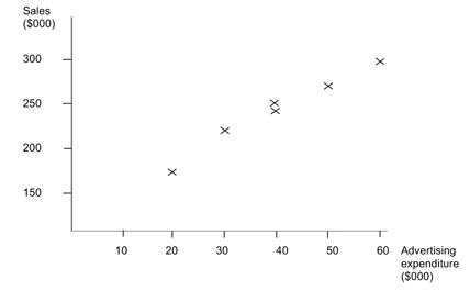
A company has recorded expenditure on advertising and resulting sales for six months as follows: Month Advertising expenditure Sales   x y   $000 $000 March 20 170 April 40 240 May 50 260 June 60 300 July 30 220 August 40 250 Required: (a)        Plot the data on a scatter diagram and comment. (b)        Calculate the line of best fit through the data, and interpret your values of a and b. (c)        Forecast sales when advertising expenditure is: (i)         $50,000 (ii)        $100,000 and comment on your answers. Solution: (a) There appears to be a positive linear relationship between advertising expenditure and sales. (b) x y xy x2 y2 20 170 3,400 400 28,900 40 240 9,600 1,600 57,600 50 260 13,000 2,500 67,600 60 300 18,000 3,600 90,000 30 220 6,600 900 48,400 40 250 10,000 1,600 62,500 240 1,440 60,600 10,600 355,000 The line is: y = 120 + 3x This means that when advertising expenditure is zero, sales will be $120,000, and for every $1 spent on advertising, sales will increase by $3. (c)(i) Sales = 120 + (3 × 50) = 270 Forecast sales are $270,000 This is an interpolation within the sample range of values and is likely to be fairly accurate. (c)(ii) Sales = 120 + (3 × 100) = 420 Forecast sales are $420,000 This is an extrapolation outside the sample range and may be inaccurate.